I thought I would look again at Pat Frank’s paper that we discussed in the previous post. Essentially Pat Frank argues that the surface temperature evolution under a change in forcing can be described as
![\Delta T(K) = f_{CO2} \times 33K \times \left[ \left( F_o + \sum_i \Delta F_i\right) / F_o \right] + a,](https://s0.wp.com/latex.php?latex=%5CDelta+T%28K%29+%3D+f_%7BCO2%7D+%5Ctimes+33K+%5Ctimes+%5Cleft%5B+%5Cleft%28+F_o+%2B+%5Csum_i+%5CDelta+F_i%5Cright%29+%2F+F_o+%5Cright%5D+%2B+a%2C&bg=ffffff&fg=333333&s=0&c=20201002)
where 


Pat Frank then assumes that there is an uncertainty, 

which assumes an uncertainty in each time step of 
 Since I’m just a simple computational physicist (who is clearly has nothing better to do than work through silly papers) I thought I would code this up. That way I can simply run the simulation many times to try and determine the uncertainty. Since it’s not quite clear which term the uncertainty applies to, I thought I would start by assuming that it applies to


The result is shown in the figure on the upper right. I ran a total of 300 simulations, and there is clearly a range that increases with time, but it’s nothing like what is presented in Pat Frank’s paper. This range is also really a consequence of the variation in
 The next thing I can do is assume that the
 Given that in any realistic scenario, the annual change in radiative forcing is going to be much less than

Pat Frank’s analysis essentially suggests that adding energy to the system could lead to cooling. I’m pretty sure that this is physically impossible. Anyway, I think we all probably know that Pat Frank’s analysis is nonsense. Hopefully this makes that a little more obvious.

Could you rerun this simulation for a few billion years? Or for the creationists for 6 thousand years? Would be interesting to see in which fraction of the runs live on Earth is possible, must be pretty close to zero.
“Pat Frank’s analysis essentially suggests that adding energy to the system could lead to cooling.”
Yes, that is the problem with these random walk things. They pay no attention to conservation principles, and so give unphysical results.
But propagation by random walk has nothing to do with what happens in differential equations. I gave a description of how error actually propagates in de’s here. The key thing is that you don’t get any simple kind of accumulation; error just shifts from one possible de solution to another, and it then depends on the later trajectories of those two paths. Since the GCM solution does observe conservation of energy at each step, the paths do converge. If the clouds created excess heat at one stage, it would increase TOA losses, bring the new path back toward where it would have been without the excess.
Nick says:
Therein lies the rub. ENSO is so clearly not a random walk and so obviously the solution of a DiffEq. The connective tissue is a stochastic DiffEq such as Ornstein-Uhlenbeck which can be considered as a random walk inside an energy well. That has a definite bound given by the depth of the well.
p.s.
Is Carl Wunsch a friend of Patrick Frank’s ?
Nick Stokes says: “Pat Frank’s analysis essentially suggests that adding energy to the system could lead to cooling.”
Yes, that is the problem with these random walk things. They pay no attention to conservation principles, and so give unphysical results.”
ATTP . “ I’m pretty sure that this is physically impossible.“
–
The comments above seem somewhat misplaced.
Adding energy to a system does cause warming of the overall system
We know it is physically impossible to cause overall cooling
So doe Pat Frank.
Therefore the suggestion that he claims that adding energy to the system could cause cooling (to the system) is wrong.
You should at least treat his argument in the proper spirit it is put forward rather than misquoting it.
Two points.
The argument is that the amount of energy received has an error range which means that the system could receive less rather than more energy , hence it could become increasingly colder.
Otherwise there could be no random walk cooler.
Second but not important is that when heat is added to a system it is not added or emitted equally so of course one part of a system can get temporarily colder if the rest overwarms.
Play fair.
It is reasonable to use a linearised approximation (e.g. Taylor series) to analyse the behaviour of a physical model, which is basically what Franks has done here. However to assume that statistical uncertainties in the approximation apply to the physical model is clearly unreasonable as the physical model may contain constraints or feedbacks that quickly limit the effect of the uncertainties. In this case I am thinking of Stefan-Botlzmann law, which means that if the Earth warms by 20C or so, there needs to be a big input of energy to compensate for the extra (fourth power) energy radiated into space.
It also ought to be obvious that a local linearisation can’t be extrapolated out a long distance, at least without some form of analysis of the stability of the approximation.
ATTP,
It is a discrete 1D random walk, PF’s plots only show the one sigma curve, for that one sigma i get:
Error (degrees C) = 1.578*SQRT(time), it is a conic (parabola) section. For reasonable N (say anything above ~20) the distro is gaussian with zero mean.
In the limit (as dt approaches zero) it is a form of diffusion equation, the diffusivity coefficient would have to be units of Kelvin^2/second.
You can do the random walk long hand for any N, but it is much faster to just use a gaussian distribution (I use the polar method) for any specific N.
https://en.wikipedia.org/wiki/Marsaglia_polar_method
The LLN/CLT dictates that the gaussian distro is exact.
I’ve been meaning to ask if anyone here uses the Ziggurat algorithm, as in Is it exact (I have some code but I need to run it a few billion times)? I already know that the polar method is exact.
Victor,
Well, if you run it for thousands of years, then you’re right that the Earth itself becomes unlikely and there is a non-negligible chance of the temperature dropping below absolute zero.
Nick,
Yes, a good point.
angech,
This doesn’t make any sense. He’s essentially applying an uncertainty to the change in forcing, but his reasoning is that this is a consequence of an uncertainty in the cloud forcing (I’ll ignore here that he’s confused the cloud forcing and the cloud feedback). Hence he is indeed suggesting that an increase in the external forcing could lead to cooling due to the uncertainty in how the clouds will respond. This is pretty nonsensical.
ATTP
It is a published paper.
With reviewers that I think you respect.
He can do maths.
We are discussing it.
In this light the claims of it being nonsensical have to address the substance of the maths and the substance of the claim, here the uncertainties in the cloud forcing.
(ATTP “I’ll ignore here that he’s confused the cloud forcing and the cloud feedback”)
* Could we agree that cloud forcing has an element of being a negative feedback or failing that that Pat Frank is certainly describing a forcing which can be negative as well as positive?
If so, then cloud cover can cause a decrease in temperature ( cooling) just as much as an increase in cooling.
Which is not nonsensical.
If your argument is that cloud forcing can only ever be positive then your opinion on it being nonsensical holds, not because of his maths but because you have denied the validity of his claim on cloud feedbacks and forcings.
So * ?
I’ve put up a post here on error propagation in differential equations, expanding on my comment above. Error propagation via de’s that are constrained by conservation laws bears no relation to propagation by a simple model which comes down to random walk, not subject to conservation of mass momentum and energy.
angech,
The cloud response is a feedback, not a forcing. It is logically inconsistent for a feedback to lead to long term cooling when the initial change in forcing lead to warming. If clouds could counteract the change in forcing, then the response should eventually return to 0 and the cloud feedback should then turn off. In this case, you’d still have the change in forcing, which was positive. Hence, the idea that the cloud response could lead to long term cooling even if the initial change lead to warming, does not make any sense.
Nick,
Very nice post. Thanks.
“ATTP
It is a published paper.”
angech, it is a paper that was reviewed and rejected 12 times before it was accepted by a journal. Failures of peer review happen, submitting it 13 times makes that very, very likely.
Say there is a 0.95 probability that a journal will reject a bad paper. Thus the probability of it not being rejected by a journal is (1 – 0.95). The probability that *all* of the thirteen journals will reject it is (assuming independent reviews) is (1 – 0.95)^13 = 1.2207e-17. Thus the probability that one or more would accept it is 1 – 1.2207e-17 is too close to 1 for it to be represented as anything other than 1 in double precision floating point arithmetic.
Less hubris please. ATTP also has a good command of maths, but also a good grasp of the physics, which is conspicuous by its absence in Franks work. Stefan-Boltzman means that cloud feedback is not going to cause 20C of warming in 100 years.
Sorry too early in the morning. it should of course be 1 – 0.95^13 which is about a 50:50 chance of a paper being accepted by one of the journals. Mea culpa. The point is that a paper being published doesn’t make it valid or correct or reliable. If you submit it thirteen times, it becomes a coin flip as to whether it gets published or not, no matter how wrong it is, and that is what Franks has done.
dm,
PF also had to pay-to-play, I think those 13 other failed attempts were to ‘so called’ real journals (no author publishing fees).
p = 1 for a paper that claims that 1+1=3, as long as you are willing to pay for it. Check it out in The International Journal of Incorrect Addition! 😉
Yes, from what I have seen, it seems that he was getting to influence the choice of reviewers as well, which alters things somewhat. Journals should *never* ask the authors to nominate reviewers, it is a recipe for pal-review and if competent editors cannot select reviewers by themselves (because they don’t know the sub-field well enough), then the paper is likely to be out of the scope of the journal.
Nick says:
The title of your post is misleading as in addition to Ornstein-Uhlenbeck there are many other stochastic DiffEq that have elements of random walk (i.e. diffusion) and higher-order natural responses to them. One in particular is Fokker-Planck, which is the ubiquitous transport equation.
The uncertainty can be in the forcing or the transport coefficients (diffusivity, mobility) and this will have a differing impact on the result depending on which terms have the error. The bottom-line is that you can’t in general get away from the random walk component.
I really don’t care what Frank is trying to compute because his initial premise is wrong, and I tend not to correct the detailed work when the premise is wrong. In the real-world, there’s no extra credit for work past this point.
Paul
“there are many other stochastic DiffEq”
I’m sure that is true. I am talking about error propagation in the Navier-Stokes equations as implemented in GCMs. I have decades of experience in dealing with them. It is supposed to also be the topic of Pat Frank’s paper.
Good posts here and by Nick. Conservation laws and other underlying physics are driving GCM results not the state of motion. Saw the paper below referenced recently by Peter Thorne. Water vapor feedback is captured well in “good” and “poor” performing GCM’s. In other words, the physics is robust to uncertainty/errors in fluid motion.
https://www.pnas.org/content/106/35/14778
Nick, The point is that whether it is Fokker-Planck or Navier-Stokes, there is an Einstein relation that connects diffusion (i.e. random walk) to mobility (or inverse viscosity w/ N-S) . But random walk in these cases is not the same as random walk in other situations since the ensemble statistics of the particles smooth out the excursions so all one sees is the average.
The analogy that the misguided effort is trying to portray is that of individual trajectories, which would be like the Black-Scholes equivalent of Fokker-Planck. That is, if one follows a individual trajectory, one can try to isolate a trend or drift from the random walk of the object. But this is misguided, as the main variability is due to ENSO anyways and this is a deterministic path with the expected ensemble averaging of the diffusional component smoothing out the excursions.
At what scales are your governing equations applicable to (geometric, kinematic and dynamic)? We already know that tides are global. Although people often use a partial domain (say North Atlantic and GOM along the eastern seaboard) with the correct deep water open ocean boundary conditions specified.
According to PF there is about a 32% chance that air temperature will vary by more than ~1.6K in any given year/ Again, I ask what does a random walk have to do with the conservation laws? Nothing!
I did a 2D random walk and consumed a lot of energy because I was really TokedOutDude while the door was only ever one step away the whole time. See that? The start of an energy conservation law.
Consider a equidistant diagonal lattice …
where t is time and x is temperature. All possible paths of N diagonal steps have the exact same path length!
If we associate the same energy consumed for a single diagonal move then all possible paths taken consume the exact same energy.
That is PF’s energy conservation law, all paths consume the exact same amount of energy. I would add that this is not a very useful energy conservation law.
https://www.researchgate.net/profile/Francesca_Colaiori/publication/1950133/figure/fig1/AS:670714738786312@1536922263731/Typical-configuration-of-m-4-friendly-walkers-on-the-diagonal-square-lattice.pbm
Everett said:
I’m not certain which discussion this is directed to, but here is Scientific Reports hot off the press.
Switch Between El Nino and La Nina is Caused by Subsurface Ocean Waves Likely Driven by Lunar Tidal Forcing
They asked the obvious question and looked at the data, which is the time-series of the predominate subsurface wave associated with ENSO. They essentially demonstrate that it’s not the Kelvin wave or wind forcing that is responsible — the consensus reasons — which leaves the only possibility left, which is Carl Wunsch’s favorite forcing for ocean transport.
Pinning this down will do more than anything else to eliminate the variable/random component, which allows the Frank’s of the world to contribute to the FUD.
@Nick Stokes Good post at your blog regarding basic numerical analysis.
angech says: “It is a published paper.”
You’re going too far with that claim.
https://en.wikipedia.org/wiki/Frontiers_Media
angech says: “With reviewers that I think you respect..”
“Frontiers has used an in-house journals management software that does not give reviewers the option to recommend the rejection of manuscripts” and that the “system is setup to make it almost impossible to reject papers.”
https://books.google.ca/books?id=dwFKDwAAQBAJ&pg=PA304&lpg=PA304&dq=journal+frontiers+predatory&redir_esc=y&hl=en#v=onepage&q=Frontiers&f=false
angech says: “He can do maths.”
“In July 2016 Beall recommended that academics not publish their work in Frontiers journals, stating “the fringe science published in Frontiers journals stigmatizes the honest research submitted and published there”, and in October of that year Beall reported that reviewers have called the review process “merely for show”.”
https://web.archive.org/web/20161127152107/https://scholarlyoa.com/2016/10/27/reviewer-to-frontiers-your-review-process-is-merely-for-show-i-quit/
angech says: “We are discussing it.”
Its a junk journal angech, pure and simple. And dude. THIS IS NOT WHERE SCIENCE IS USED. You got that? Scientists publish to communicate to other scientists. Do you understand that very very basic principle behind publishing scientific papers? The only way his paper will prove itself is if you see a slew of scientists applying his new and novel theories to their own work. Judging by the actual public from real scientists… His paper was born on the fringes, and is still born.
I note at this point that Roy Spencer has also written a blog post on this paper, basically agreeing with the major argument of Stokes:
https://www.drroyspencer.com/2019/09/critique-of-propagation-of-error-and-the-reliability-of-global-air-temperature-predictions/
Windchaser,
Yes, I also noticed that even Roy Spencer doesn’t agree with Pat Frank’s analysis. I wonder what names Pat is going to call him?
Another way to think about this problem: pretend one of the GCMs is actually the “real world”, and the other 40 are all emulations of that GCM. There will be almost exactly the same average error in radiative forcing between the “real” GCM and the “emulations” as there is between the GCMs and the real Earth. So why don’t all the GCMs diverge in a Frankian manner from the “real” one? Because Frank is dead wrong. And no scientist worth his salt should take more than 30 seconds to realize that the paper isn’t worth the paper it isn’t printed on. It is truly embarrassing for the journal, and for any reviewers who didn’t recommend immediately throwing it into the circular file.
I read Dr. Roy Spencer’s post with great interest. I also read Dr. Pat Frank’s comment in response. I am leaning toward Spencer – but confused about the +- 20 unit issue. Pat says the +- 20 isn’t temperature, which Roy took it to be. Didn’t read hard enough to figure out what the units are for the +-20 (or is it unitless?). Anyway – this is interesting (to me at least).
Richard,
Pat’s just talking more and more nonsense. If it isn’t temperature what is it? His equation for temperature evolution is:
Clearly the term has unit of K and is clearly the term he then propagates. To claim that it’s some uncertainty statistic, and not a temperature, is just nonsense. Uncertainties represent something real (i.e., they represent the range of possible results). They’re not some kind of statistic that doesn’t represent something real.
I knew Frontiers were a bit of a shady multi level marketing scheme, but that it is not possible to recommend rejecting a paper is amazing. And after that they publish the article with your name as reviewer on it and in doing so destroy your scientific reputation. Thanks for the warning.
Richard,
“Anyway – this is interesting (to me at least).”
Which aspect is interesting? (Genuine question)
VV,
“And after that they publish the article with your name as reviewer on it”
No, I think the options are submit a recommendation to publish, or don’t submit a recommendation at all. In this case Carl Wunsch and Zanchettin submitted recommendations to publish, and their names are listed. The other two referees did not.
Nick, good. I still will not review for them.
So that is another two reviewers for the computation of dikranmarsupial. In a normal journal, two rejections and you are dead.
PF: “I’m sorry Roy. You’ve made one very fundamental mistake after another. Your criticism has no force.”
Translation: You all are just steaming barking mad that I discovered the real error first…

I wouldn’t want to submit articles for a journal where the reviewers cannot unequivocally reject a paper. Any reviewer that rejects my paper when I am wrong (which does happen, no matter how hard you try – we are only human) is a good friend to me and has my best interests at heart (if they didn’t they’d be happy to see me destroy my academic reputation).
Not going to review or submit to Frontiers.
Richard Arrett says: September 11, 2019 at 9:26 pm – I read Dr. Roy Spencer’s post with great interest. . .
What I found most interesting thing about Dr Spencer’s post is that is that it wasn’t until the 24th paragraph* that Spencer gently said Frank was talking nonsense after having aired his own grievances about the barriers to skeptics getting published** and climate modeling in general.
This rather speaks to the problem of the “red team” review in that there seems to be little coherency in what the red team believes except that AGW isn’t a problem.
* – 24th paragraph in the first version I saw, it’s been revised at least twice since
** – difficulties of skeptics getting published – a bit weird to tie this in with a review of a deeply flawed paper
ATTP: Aren’t models ensemble means of simulations? The reason I ask is that averaging different runs is done to remove random error. Its how we clean up data.
You pointed to VVs bit in 2015;
http://variable-variability.blogspot.com/2015/09/model-spread-is-not-uncertainty-nwp.html
AoM,
I think the problem is that what’s presented isn’t really an ensemble of one model with a range of initial conditions and with a range of possible input parameters. It’s a whole mixture of models. Hence the range is a representation of uncertainty, but isn’t really a formal uncertainty (it doesn’t consider all possible sources of uncertainty). At least, I think that is roughly right.
ATTP: So… if you had error in such a system, then it would be reduced. Just humor me and average all the runs of your forcing graph. (Yeah I get this isn’t kosher, but then neither is Pat Frank pretending simulations are single runs with massive wide error.)
AoM,
I’m not sure I follow what you mean by “it would be reduced”? If I average all the runs of my top graph, it would fall right in the middle.
yup.. In 100 years it would be right in the middle…
I think it is important to bear in mind that the ensemble mean is not directly a (conditional) prediction of the observed evolution of the real climate, but only of the forced component of the real climate (because the chaotic internal variability that depends on the initial conditions will be averaged out as well, but it will still be present in the observed climate).
dirkran… (not that I want to propagate nonsense…)
I know.. I just just that a lot of folks look on simulation output as though its some sort of single factual run. But it really isn’t. Although that is how current temperatures are compared against simulation runs.
The reason for executing multiple simulations (an ensemble), is in part to average out error. It also gives us information about standard deviation, etc.
(I guess I can just drop this…)
Good to spar, better to let others do it for you. Watching Roy v Pat with great interest.
Plus comments here.
Takeaway so far is Pat contending that he is just showing the propagation of systemic error in GCM’s quite different to random error which both Pat and an oilman point out would tend to disappear with more runs.
Mathematically the systemic error or its root mean square used by Pat over a 65 year period has to lead to a large positive and negative uncertainty range as he shows.
He specifically states it is only the maths in computer models not the physics that he is discussing not the real or observational world.
Mathematically this is sound.
Practically it’s relevance is debatable but it does open up a can of worms about the way computer programmes now project uncerainty into the future.
Unless this is specifically addressed and tightened up by the programmers, Mosher would agree as he supports more open coding, and we can all see the assumptions and uncertainties going into these programs then Pat is free to make his comments and those disagreeing need to show that their programmes do not have the systemic bias in he seems to have identified.
Seems Pat Frank has been at this for over a decade. Some good responses from the realclimate crowd at the time: http://www.realclimate.org/index.php/archives/2008/05/what-the-ipcc-models-really-say/comment-page-9/#comment-95545
lerpo,
Yup, but back in 2008, it was a linear with time propagation error ,,,
Click to access climate_of_belief.pdf
Good find, lerp.
I especially like this inline comment from Gavin:
“Response: Ummm… a little math: log(C/C0)=log(C)-log(C0). Now try calculating log(0.0). I think you’ll find it a little hard. indeed log(x) as x->0 is undefined. What this means is that the smaller the base CO2 you use, the larger the apparent forcing – for instance, you use CO2_0 = 1 ppm – but there is no reason for that at all. Why not 2 ppm, or 0.1 ppm, or 0.001 ppm?”
http://www.realclimate.org/index.php/archives/2008/05/what-the-ipcc-models-really-say/comment-page-9/#comment-95789
Remind anyone of the arbitrary 1-year period Franks uses in his paper?
@anoilman There is a good discussion of the meaning of the ensemble here
http://julesandjames.blogspot.com/2010/01/reliability-of-ipcc-ar4-cmip3-ensemble.html
I find it hard to understand how the IPCC continued with the “truth centred” interpretation of the ensemble rather than the “statistical exchangabiloty” interpretation, as the former is obviously wrong (consider an ensemble of “perfect” earths, e.g. Earths from parallel realities with similar forcings).
In statistical mechanics, an ensemble is used because that’s the way we understand the physics.
In climate science, an ensemble is used as a crutch because we can’t isolate the true physics.
Having said that, I seriously think we can do better. If I didn’t, I wouldn’t be working on the challenge.
So James Annan says the following view is implausible, because we can never know the “truth”:

For comparison, I played a game of darts with respect to this grand-scale geophysics topic earlier this year: https://geoenergymath.com/2019/02/13/length-of-day/
How close to the bulls-e can we get this? At some point, we realize that we are hitting the bulls-eye directly and then it’s a matter of piling on 2nd-order effects to finish it off and claim victory.
Why can’t this be done for climate variability? Nothing says it can’t.
Paul,
The problem is that the intrinsic variability means that the range could represent the range of actually physically plausible pathways, rather than simply representing an uncertainty around the actual pathway. If we have a perfect model, and chaos was not a problem, then maybe we could determine the actual pathway, but we probably can’t. Hence, we shouldn’t necessarily expect the ensemble mean to represent the best estimate of reality.
“I find it hard to understand how the IPCC continued with the “truth centred” interpretation of the ensemble rather than the “statistical exchangabiloty” interpretation”
If you formulate it like this, the IPCC position makes perfect sense communication-wise. 😉
said:
Chaos is the other crutch. If you look at the analysis of the geophysics problem that can be accurately modeled, that of LOD, you will realize that is a simple rigid-body response. That’s of course straightforward to represent as a direct forcing. But climate variability is a non rigid-body or fluid response to a forcing. This only has the complication that the response is non-linear, and that non-linearity can be accommodated by solving Laplace’s Tidal Equations (aka the GCM’s) properly.
I seriously think we can do this, and from my earlier comment above #comment-162350, I am not alone in this opinion.
…and Then There’s Physics
“The problem is that the intrinsic variability means that the range could represent the range of actually physically plausible pathways, rather than simply representing an uncertainty around the actual pathway. If we have a perfect model, and chaos was not a problem, then maybe we could determine the actual pathway, but we probably can’t. Hence, we shouldn’t necessarily expect the ensemble mean to represent the best estimate of reality.”
Thanks for this refreshing bit of reality.
Also I see.
“James Annan says the following view is implausible, because we can never know the “truth”:
–
This sums up the Pat Frank controversy.
He is pointing out that the way we do things still has lots of potential errors in them.
This means that there is a small chance that the arguments for AGW may be wrong.
Shooting the messenger is not the right response.
Improving the understanding as Paul suggests is the correct way to go.
People should be thanking him for raising the issue and addressing his concerns on their merits. Then doing the work to address the concerns.
–
My worry is that if he is correct the models have a lot more self regulating in them addressed to TOA than they should which in turn makes them run warm.
angech,
Pat Frank is wrong. He is definitely wrong. You really don’t need to worry. What Pat Frank has presented has little bearing on reality, let alone on how climate models actually work.
PP “In climate science, an ensemble is used as a crutch because we can’t isolate the true physics.”
No, that is incorrect. Say we had access to an ensemble of Earths in parallel dimensions (and a time machine), were the forcings were identical and only varied in their initial conditions. You could make no better model of the Earth than another Earth. The physics would be exactly the same, and the temporal and spatial resolution would be effectively infinite (Planck length/time). You could STILL expect no better than for the actual Earth’s climate to lie in the spread of the ensemble somewhere, and to be no closer to the ensemble mean than any individual member of the ensemble. That is why the “truth-centered” interpretation is wrong (unless you understand it to be an estimate of the forced component of the observed climate change, rather than just the observations).
angech wrote “This sums up the Pat Frank controversy.
He is pointing out that the way we do things still has lots of potential errors in them.”
No, he is pointing out an error that doesn’t accumulate in the models (or reality) in the way that he suggests. It is obvious to anyone with a reasonable grasp of physics to see that.
“Shooting the messenger is not the right response.”
No messengers are being shot. It is Frank’s message that is getting shot down, not Frank (except for his inability to listen to those patiently explaining his errors, but that is pretty reasonable IMHO).
“People should be thanking him for raising the issue”
no thanks are due for raising in incorrect error and not listening to the explanations of why the issue is not correct.
“and addressing his concerns on their merits.”
They have been addressed on their merits. They have none, for the reasons that have been explained multiple times. For instance by the reviewers of 12 journals.
“Then doing the work to address the concerns.”
No work is neccessary as the concerns have no merits.
If you disagree, present your evidence.
Let me preface this by mentioning that Carl Wunsch is also at the center of this controversy, since he OK’d Frank’s paper to be published. Wunsch has written extensively on the theory of tides, and while no one questions that we can establish the true physics of conventional tides, like him, I would suggest that tidal forces have a wider impact than the consensus would suggest. Read his Nature paper from 2000 titled Moon, Tides, and Climate.
With that, consider we had an ensemble of earth/moon/sun systems with identical orbital configurations. I would suggest there would be no difference in the resultant tidal responses. It is well known that the quiescent tidal responses are independent of initial conditions and thus are a pure forced response (once the natural response dies out). So each instance within the ensemble would align with the others, making the ensemble unnecessary. All we have to do is calibrate the model to an observational interval and we are good to go with the single instance to accurately represent the true physics.
All I am suggesting with my own model of ENSO, is that the long-period tidal forces impact the oceanic thermocline similarly and that this behavior is as deterministically non-chaotic as conventional tides. When this reaches a quiescent steady-state, the concept of an ensemble is no longer necessary, just as it is not necessary to do generate an ensemble of conventional tidal simulations to construct a tidal table.
This is a narrow topic and I am not suggesting that this is true for more localized weather simulations, where the outcomes are clearly dependent on starting conditions.
I am only guessing but perhaps Wunsch is frustrated by the status quo in understanding climate variability and he wanted to shake things up in his retirement years? I am all for that but am still puzzled by why he would use P.Frank to fly that flag.
This has been a most fascinating read, including many of the old posts that people have linked to. I have to admit, it has been a very long time (or never) since I have seen someone argue for so long from a position that is so wrong as Pat Frank.
The most intriguing thing has to be the units associated with the whole “W/m^2 over one year” thing. Has anyone ever pointed out to him that Watts are already a rate? That Watts are not a quantity of energy, but a transfer of energy per unit time? I mean, a Watt is still defined as a Joule per second, isn’t it? Or has someone overturned that part of physics when I wasn’t looking?
Bob,
People have pointed out many things to Pat Frank, all without much success. Not sure if they’ve pointed out that specific issue, but I suspect someone must have.
Paul Pukite (@WHUT) says
“With that, consider we had an ensemble of earth/moon/sun systems with identical orbital configurations. I would suggest there would be no difference in the resultant tidal responses. It is well known that the quiescent tidal responses are independent of initial conditions and thus are a pure forced response (once the natural response dies out). So each instance within the ensemble would align with the others, making the ensemble unnecessary. All we have to do is calibrate the model to an observational interval and we are good to go with the single instance to accurately represent the true physics. the long-period tidal forces impact the oceanic thermocline similarly and that this behavior is as deterministically non-chaotic as conventional tides. When this reaches a quiescent steady-state,”
–
I feel the gods of chaos would interfere more than you are giving credit for. There is more to it than just the large scale dynamics you mention. Local factors include organic changes such as ocean blooms, forestation changes over millions of years where minute variations in propagation circumstances could lead to altered rainfall and water storage changes. Also both meteoritic and volcanic activity cannot be assumed to be identical over time. (Perhaps the former if you are being deterministic enough).
The resulting changes in tidal patterns will persist for eons even if eventually at a minuscule level. No matter what pattern you ascribe the fluid dynamics mean major or minor currents can develop many years or centuries later and move in perhaps the opposite way to what you expect.
I think it is good you can build up a theory and use it generally well in practice but it needs to be a dynamic system which resets itself after each developing vagariety.
Bob,
“Has anyone ever pointed out to him that Watts are already a rate? “
No, the actual nature of the units are not the issue. If the quantity really was increasing by x units/year, then the /year would be appropriate, whether units were watts or whatever. But they aren’t. They are just annual averages, as you might average temperature annually. That doesn’t make it °C/year.
angech said:
” Local factors include organic changes such as ocean blooms, forestation changes over millions of years “
angech forgetting the skeptic slogan “all other things being equal”.
“The resulting changes in tidal patterns will persist for eons even if eventually at a minuscule level. No matter what pattern you ascribe the fluid dynamics mean major or minor currents can develop many years or centuries later and move in perhaps the opposite way to what you expect.
I think it is good you can build up a theory and use it generally well in practice but it needs to be a dynamic system which resets itself after each developing vagariety.”
Is angech one of the rare Aussies that doesn’t live next to the ocean? Tidal patterns have never been known to go out of phase with their forcing. I thought it was common knowledge among sea-side dwellers that tsunamis, cyclones, etc will not impact the patterns after the disturbance dies down.
angech can always be guaranteed to give the naive take, so I guess that’s good in a way.
If he believes the units for an average are x per year, it would be interesting to hear what units he thinks a standard deviation should have. Or, for that matter, a RMSE.
John,
Indeed. In fact, I think the value he is using is actually the RMSE.
In fact, John had a nice Twitter thread about the Frank paper.
Paul,
I remain amazed at how the people who do the tides get it so right and have done so for many years which proves your point about the patterns.
Used to live in Darwin where the tides would go out kilometres and come back in.
All other things being equal is good for mechanical forcings and predestination but I do not think models can forecast volcanoes and organic factors. Once you let any vestige of chance occur the potential effect on the patterns could be important and unpredictable at times. As you point out there is a lot of stability in the system.
AYP, John,
PF is using something called the square root of the root sum square (no division of the sum as one would do for RMSE).
An error function that starts out as orthogonal to the time series at t = 0 (infinite slope).
On another matter, how is it that we can reasonably accurate calculate GMST with only about 60 gauges? I know that ATTP has had at least one blog post in that regard. Now, I think that error improves as the (inverse) square root of the number of gauges. The average is twice as accurate for N = 3,600, not proportional to the square root of N but proportional to the inverse square root of N.
“(no division of the sum as one would do for RMSE)”
should read …
“(no division of the sum by N (number of observations, in this case N = years) as one would do for RMSE).
angech said: “but I do not think models can forecast volcanoes”
Yet volcanoes (along with solar eclipses) are factors that provide a means to calibrate models. Scientists know precisely when they occur and can gather data on the emission impulse and then characterize the impulse response. So if it wasn’t for the other natural variability (ENSO) getting in the way, having only volcanoes dotting the historical time-series would have allowed a large reduction in the size of the ensemble needed for backcasting. A good example of this was the 1982 El Chichon volcano coinciding with the 1982-1983 El Nino — that was a wash in terms of calibration as the two events essentially cancelled. The bottom-line is that having a better model for ENSO would help the overall modeling tremendously — which isn’t saying anything controversial.
Paul
“ The bottom-line is that having a better model for ENSO would help the overall modeling tremendously — which isn’t saying anything controversial.”
Agreed.
ATTP:
Oh, based on his participation on other blog postings, I have no illusions that anything would reach Pat Franks. Maybe it would influence some of the individuals that think his ideas have some merit, though.
Nick:
…but now you are talking about the rate of change – i.e., the next derivative with respect to time. Of course that will have an additional “per unit time” term in the units. The slope of a straight line doesn’t change because you looked at it using a finite difference method (average between two points) instead of using the derivative at a single point. That’s the level of idiocy in Frank’s work.
“The bottom-line is that having a better model for ENSO would help the overall modeling tremendously — which isn’t saying anything controversial.”
yup
dikranmarsupial, if you still are watching…. Can you guess what legitimate interpretation of uncertainty might be what Frank is distorting? I’m asking you because of your commenting on frequentist versus other interpretations of probabilities on various blogs. Frank seems to be insisting that the uncertainties he is (incorrectly) computing are not uncertainties in temperature, have no relationship whatsoever to temperatures in the real world, and have no relationship whatsoever to model results no matter how many model runs are done and no matter the changes in the inputs or anything else about the models. I am baffled where he is getting these ideas.
Tom, I have no real idea what Franks means by uncertainty here – if it has no relationship with the real world and doesn’t describe what the models actually do, then it is hard to see any framework in which it is meaningful. I suspect it is one of those “if your only tool is a hammer” situations, where someone is familiar with error propagation in one problem and then applies it to another without properly investigating whether it is another nail or a hex-head bolt.
BTW Nick Stokes has a very interesting looking post at WUWT (who do occasionally post goog articles) here. The appendix sums up my main objection to Frank’s analysis (other than it is obviously non-physical):
[emphasis mine]
Tom,
I think he is taking a perfectly reasonable error propagation method (that you would apply if you were combining a number of measurements each of which had errors) and applying to a situation where it really doesn’t apply. Nick Stokes has a nice post about error propagation in GCMs.
Tom sez …
“I am baffled where he is getting these ideas.”
AFAIK, it originated with the firm belief that a GMST anomaly can not be calculated because of instrument bias errors, essentially that the mean error is assumed to be zero and Gaussian distributed, but due to bias errors it can not be zero mean and Gaussian distributed..
Yet a 1D discrete random walk is zero mean and Gaussian distributed.
Therefore, the real errors must be much larger then even a 1D random walk.

NS (at WUWT!) finally sez …
“Root sum square with uniform terms (as here) implies iid random variables. That is, independent, identically distributed. Independence is a big issue. In the PF mark ii paper, there was talk of autocorrelation etc in Eq 4, but it all faded by Eq 6. And necessarily so, because the datum was a single value, 4 W/m2 from Lauer. But identically distributed is the issue with DEs. Successive errors are not identically distributed. They are modified by the progress of the DE.”
Which is the answer I got when looking into the issue yesterday. Is what we are modeling, a stochastic process and/or a deterministic process? Both until you measure it.
A deterministic process has perfect autocorrelation!
As to the 4 W-m^2 issue, consider it a time invariant number (same value at 400 years as at 20 years), what then is the RMSE? Zero.
sqrt(4/0)=infinity
sqrt(4/1)=2
sqrt(4/20)=0.44
sqrt(4/400)=0.1
sqrt(4/infinity)=0 (time invariant)
Corrections welcome.
If 4 W-m*2 has a non-zero RMSE then what does one do? Plot the residuals and find the distribution, if it looks Gaussian with a mean, then state the mean and sigma. Basically find the distribution.
Even more corrections welcome.
Everett
“As to the 4 W-m^2 issue, consider it a time invariant number (same value at 400 years as at 20 years), what then is the RMSE? Zero.”
4 W/m-2 has a time component hence it is a time codependent “issue” for want of a better term.
You now extrapolate it over 20 or 200 years and claim it is invariant.
It can only be a constant if it has no standard deviation.
Can you explain what you consider the 4 W/m-2 to be?
You the complicate matters by saying
“If 4 W-m*2 has a non-zero RMSE” and talking about residuals which can only happen with some degree of standard deviation or a non time invariant number.
DM saw that comment too.
“Sharing a common solution does not mean that two equations share error propagation. So it’s not OK.”
The logic is not correct. It can also mean.
“Sharing a common solution can mean that two equations share error propagation.”
In which case it could be OK.
The question Nick avoided was if the two equations do share error propagation.
In his answer on one of the special equations he gave he made it quite clear that if the special equation did have perturbations (SD or “error”) it would give a random walk which of course inevitably leads to Pat Franks conjecture.
ATTP sums it up thus
“I think he is taking a perfectly reasonable error propagation method (that you would apply if you were combining a number of measurements each of which had errors) and applying to a situation where it really doesn’t apply.”
And you said it was one of those “if your only tool is a hammer” situations.
angech “The question Nick avoided was if the two equations do share error propagation.”
it is obvious that they don’t and the appendix to Nicks article could hardly have spelled that out more explicitly, as I pointed out upthread. Nick didn’t avoid the question, and you owe him an apology IMHO for the accusation.
To be clear, if Franks wants to use his analysis based on a linear approximation to criticise the models, then the onus is on HIM to show that the error propagation method applies both to the approximation and the GCMs. But he does not do that, and indeed cannot do that as it is obviously incorrect. In his analysis, any error results in temperatures diverging without apparent limit. That simply isn’t physically plausible (Stefan-Boltzmann for one thing).
Actually.. what does it look like when you hind cast?
Perhaps we should the resultant graph the Dumbbell graph?
ATTP
Don’t mind if you remove this as it is a link to a post of Pat Frank at your non favourite site,
However he probably has it up at his site wherever it is and explains how he sees his reasoning.
Ta
Pat Frank September 15, 2019 at 8:00 pm
“For the benefit of all, I’ve put together an extensive post that provides quotes, citations, and URLs for a variety of papers — mostly from engineering journals, but I do encourage everyone to closely examine Vasquez and Whiting — that discuss error analysis, the meaning of uncertainty, uncertainty analysis, and the mathematics of uncertainty propagation.”
Angech, it’s patent nonsense. More explanation of nonsense really won’t help.
angech,
See physical constants …
Physical constant
https://en.wikipedia.org/wiki/Physical_constant
For example, in a shipload of applications g~9,81 m.sec^-2 ~ constant. One does a double integral (in time and strictly speaking in a vacuum) to determine the distance an object falls at any time, t.
The very nature of RMSE suggests that measured at a high enough frequency (or low enough frequency for large time), g or gravity, is strictly speaking not a constant. So, g or gravity, will have frequency (or inverse of time) response characteristics
For mass, in Earth’s gravity field,,one usually measures on a balance beam to take out the local effects of that gravity field.
PF assumes that the 4 w-m^2 is independent of all other uncertainties, PF uses an RMSE estimate over 20 years as an annual error estimate, Both of these are wrong. An AOGCM will have an uncertainty consummate with the overall uncertainty of climate sensitivity (e. g. 3C +/- 50% at equilibrium at a 90% confidence level, per IPCC AR5 WG1).
vtg,
Yes, absolutely.
Re: A Hex-headed bolt:
“For the benefit of all, I’ve put together an extensive post that provides quotes, citations, and URLs for a variety of papers — mostly from engineering journals, but I do encourage everyone to closely examine Vasquez and Whiting — that discuss the use of a hammers to drive in nails, the meaning of hammering, and the use of cross-pien or “warrington” hamme.”
90% above might need to be 66% (can’t quite remember the three conditionals at the moment, but I think they are: 66% between 1.5C and 4,5C, up to 5% below 1.0C, up to 10% above 6C, I think that is right).
66% between 1.5C and 4,5C
should read …
“minimum of 66% between 1.5C and 4.5C”
This nonsense dies with PF, thankfully.
angech,
PF assumes an infinite rate at t=0. As I stated in the previous thread, as VV suggests above and as anoilman implies above, move that parabola backward in time, it makes absolutely no sense whatsoever.
I have a three century old MIG thermometer, I stick it in boiling water, it sez 100C, I stick it in freezing water, it sez 0C. So, do I believe the three century old MIG thermometer or do I believe the error range is now +/- 1.578*sqr(300) ~ 27C for one sigma (68%) confidence.
According to PF, at the 95% confidence level, I don’t know if I am measuring solid or liquid or gaseous water.
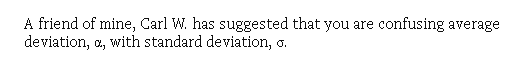
There’s a comment from Carl Wunsch on PubPeer related to this paper. I reproduce it here:
“I am listed as a reviewer, but that should not be interpreted as an endorsement of the paper. In the version that I finally agreed to, there were some interesting and useful descriptions of the behavior of climate models run in predictive mode. That is not a justification for concluding the climate signals cannot be detected! In particular, I do not recall the sentence “The unavoidable conclusion is that a temperature signal from anthropogenic CO2 emissions (if any) cannot have been, nor presently can be, evidenced in climate observables.” which I regard as a complete non sequitur and with which I disagree totally.
The published version had numerous additions that did not appear in the last version I saw.
I thought the version I did see raised important questions, rarely discussed, of the presence of both systematic and random walk errors in models run in predictive mode and that some discussion of these issues might be worthwhile.
CW”
https://pubpeer.com/publications/391B1C150212A84C6051D7A2A7F119#5
Marco,
Very interesting, thanks.
Dr. Wunsch essentially agreed with what I summarized on the PubPeer review — i.e. that the premise of the paper was wrong ” that a temperature signal from anthropogenic CO2 emissions (if any) cannot have been, nor presently can be, evidenced in climate observables”.
The rest of the paper was therefore not worth addressing, as even if Pat Frank had done all the math correctly he wouldn’t be able to support this absurd assertion.
Frank’s responses are interesting, because if he is correct, Wunsch is either lying, or he didn’t read the paper very well…(which would explain why he didn’t see the issues).
Marco,
Yes, Pat Frank’s responses are interesting.
PubPeer is often used to detect doctored images and replicated data in bioscience research papers. In that regard, the guilty parties have no other option than to apologize or go in a corner to hide and hope they can revive their career. In this case of pure BS, the guilty part will continue with endless Trump-like nonsense no matter what’s been debunked. They have nothing to lose apparently.
@VictorVenema
Not sure about the source you mention re Frontiers. Reviewers can of course recommend rejection at any stage of the review process. They can’t reject a paper themselves, that is the role of the handling editor – as it is in all journals I know.
I hope he knows that his rude and dismissive responses to criticisms are likely to be percieved as suggestive of Dunning-Kruger, rather than genuine expertise. In my experience, very few genuine experts behave that way (for a start, the don’t need to). He is very unlikely to convince anyone that doesn’t already think he is right that way.
This paper just got retracted because of improper error bars:
This is too bad since Nic Lewis initiated his criticism by asserting that “that all of the paper’s findings are wrong“. It was actually a novel technique for estimating OHC and now the novelty is no longer documented.
Contrast to Pat Frank.
Paul,
https://www.nature.com/articles/s41586-019-1585-5
“Shortly after publication, arising from comments from Nicholas Lewis, we realized that our reported uncertainties were underestimated owing to our treatment of certain systematic errors as random errors. In addition, we became aware of several smaller issues in our analysis of uncertainty. Although correcting these issues did not substantially change the central estimate of ocean warming, it led to a roughly fourfold increase in uncertainties, significantly weakening implications for an upward revision of ocean warming and climate sensitivity. Because of these weaker implications, the Nature editors asked for a Retraction, which we accept. Despite the revised uncertainties, our method remains valid and provides an estimate of ocean warming that is independent of the ocean data underpinning other approaches. The revised paper, with corrected uncertainties, will be submitted to another journal. The Retraction will contain a link to the new publication, if and when it is published.”
Everett, that’s good to hear.
Oh well, I tried over at pubpeer, but just got endless Gish gallops and questioning my educational background rather than answers to my questions (that weren’t just repeating his initial statements).
Dikran,
I tried to comment on PubPeer, but couldn’t remember my password. Probably a blessing in disguise.
A blessing indeed! Amusing that he kept going on about how I don’t understand predictive uncertainty – obviously hadn’t checked out my publications to find out my background before questioning it. ;o)
Franks is now using a comment from an anonymous denizen (“nick”) of WUWT as evidence that there exist “actual scientists” that understand his work.
I’ve given in and posted a comment (I finally realised that I was using the wrong email address).
I predict he will issue an ad-hominem about your education and reject your criticism.
Maybe if I signed it “actual scientist” that would help?
LOL ;o)
well, who could have predicted that?
I can at least relate to some of the concerns.
Consider that you were complaining about a loud erratic hum coming out of your audio device, and no one you ask seems to have any idea what is causing it. All you are told is to not worry and try to ignore it because they think the loudness is bounded. Of course it’s bounded because the audio is limited in its power output.
In climate the loud erratic hum is ENSO. Looking at hundreds of years of proxies, it seems to be bounded in its excursions so it will likely stay that way. Never mind the fact that we can’t model ENSO very well and don’t fundamentally understand what’s causing it — maybe a shift in the winds, perhaps something else.
Oddlly enough, as I am writing this, on the NJ radio station they are talking about the legend of the “Bayonne Stench” in the 1960’s. This permeated Staten Island for awhile, no one could figure it out and everyone just assumed it was coming from Bayonne.
[Patrick Frank]
I think we may have reached peak absurdity.
Dikran,
I thought we’d reached that a little while ago 🙂
I’d obviously habituated to my environment ;o)
Could I suggest it might be bed time?
vtg,
The old ones are always the best 🙂
VTG – about a decade ago ;o)
[Patrick Frank]
Peak hubris? ;o)
Pingback: 2019: A year in review | …and Then There's Physics
Pingback: How to Cavil Like Cranks | …and Then There's Physics
Pingback: Jordan Peterson: A Case Study in Sophistry and Pseudo-Profound Bullshit – The Critical Thinking Academy