I’ve written before about stabilising temperatures; stabilising temperatures requires getting net anthropogenic emissions pretty close to zero. See, for example, this Realclimate post, or Solomon et al. (2008). Stabilising atmospheric concentrations, however, would not require getting emissions to zero, but would still require substantial emission redutions (see this Steve Easterbrook post).

credit : xkcd
It should be fairly clear that what is being suggested is wrong; we’re dealing with a coupled system, so if you add new material to one of the reservoirs, it will rise in all reservoirs. However, there is a more formal way to show this. I recently worked through the ocean carbonate chemistry. It turns out that there is a factor called the Revelle factor, which is simply the ratio of the fractional change in atmospheric CO2, to the fractional change in total Dissolved Inorganic Carbon (DIC) in the oceans:
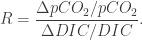
The Revelle factor is about 10, which means that the fractional change in atmospheric CO2 will be about 10 times bigger than the fractional change in 
Now, maybe if the fractional change in 
There is, however, something I’m slightly glossing over, so will try to clarify a little more. The above is based on an equilibrium calculation. In other words, it is the changes once the system has retained a quasi-steady equilibrium. Our emissions are continually pushing the system out of equilibrium and so the fractional change in atmospheric CO2 is actually greater than what the Revelle factor would suggest. Given what we’ve already emitted, we would expect about 20% of our emissions to remain in the atmosphere, but it’s currently more like 45%. This is because the timescale for ocean invastion is > 100 years, and so the system hasn’t yet had time to return to equilibrium.
Therefore, the Revelle factor is – in some sense – a lower limit; if we continue to emit CO2 – even at a constant rate – we’d expect at least 20% of what we emit to remain in the atmosphere and, hence, atmospheric concentations will continue to rise. So, unless Clive can find some problem with basic carbonate chemistry, his claim that stabilising emissions will stabilise concentrations is simply wrong.

Whilst we’re on the topic of cartoon physics:
Stabilising emission mean stabilizing the time derivative of atmospheric concentration. So the atmospheric concentration, which is its integral, should increase linearly. This assumes that processes which remove the stuff from the atmosphere are much slower. Isn’t it basically just that? (…talking as a physicist)
I.J. Khanewala, . The cumulative emission is given by
I think that’s a bit too simple. If emissions stabilise, then
So, cumulative emissions rise linearly. If the airborne fraction emains constant, then atmospheric concentrations would also rise linearly. However, the reason the airborne fraction is constant is probably because emissions have been rising almost exponentially, while each pulse of emission should decay exponentially (to give a net constant airborne fraction). If emissions are constant, then the airborne fraction should drop with time, but be limited by the Revelle factor (at least 20%).
“This, according to Clive, is something that Climate Scientists don’t yet understand.”
To misquote Einstein slightly “There are only two things that are infinite, the universe and human hubris, … but I am not sure about the universe”. The frequency with which climate blogs present overly simplistic analysis, without first bothering to do their homework and find out what scientists working on the problem have actually done already, is profoundly disappointing. Only today I see that WUWT has yet another post on the short term correlation between the annual increase in atmospheric CO2 and temperature (i.e. the Humlum/Spencer/<a href="https://skepticalscience.com/salby_correlation_conundrum.html"Salby etc. confusion) as if Bacastow had never studied this in the 1970s and nobody had ever cited his work since (of the few peer reviewed articles discussing this did not have peer-reviewed comments papers explaining why the argument is incorrect). To suggest that the climate scientists don’t yet understand the basic nature of the carbon cycle though is just ridiculous.
Skepticism is great, but it ought to start with self-skepticism.
I coded up the Bern model. The black line is using RCP4.5 emissions. The red line is constant emissions from 2020.
It seems to me to be common sense that if you disagree with a model put together by specialists who have studied the area for many years, then they may know something you don’t, so the key question is why does the Bern model (or an approximation of its impulse response) differ from your model. If you find the reason for the difference is incorrect, then you may be able to argue that the Bern model is wrong, but until then the assumption should be that you are missing something.
Best may once have been a subatomic particle physicist, but on a range of Earth and atmospheric science topics that he blogs about he’s just a half-informed dilettante.
Mrs Black has been found dead in the library and multiple lines of evidence have been discovered by others, pointing to the murder having been committed by Colonel Mustard. As a newcomer looking at the case for the first time, it’s not enough to come up with an alternative theory to explain that, in fact, Professor Plum did it. First you need to show, convincingly, why the evidence already established—and which everyone else is satisfied points to Mustard—is being either misunderstood or misinterpreted. Only then can that evidence be rejected or reinterpreted to back your alternative theory for Mustard’s innocence and Professor Plum’s guilt.
I accept that Clive Best is not denying climate change, but he might as well be, given that he’s suggesting we can carry on burning fossil fuels at the current rate.
The Revelle factor then seems to be the argument against a stabilisation. On the other hand about half the take up (sink) of anthropogenic CO2 is on land (soil & vegetation) and in the oceans by cyanobacteria/phytoplackton. I must admit I have little knowledge on Ocean Chemistry but Ferdinand Engelbeen has. This is what he wrote :
So it just takes longer. He also thinks equilibrium would be reached but at a higher level – 560 ppm.
dikranmarsupial
Does the Berne model explain then why the airborne fraction = 0.5 ? If not why ?
Clive,
Then why did you not familiarise yourself with it before making strong claims about others not understanding this topic. For example, in this post, you say
The reason is – as I understand it – because the oceans cannot simply take up all of our emissions because they’re limited by the Revelle factor. There is a reason, but you didn’t seem to bother to try and find out what it was before claiming that climate scientists don’t yet understand.
Ferdinand Engelbreen is normally quite well informed about this topic, but I’m not convinced that he’s correct about the significance of the Revelle factor. Since we’re quoting people, here’s a quote from Archer et al.:
So, on the scale of hundreds of years, 20-30% of our emissions remain in the atmosphere. On the scale of a few thousand years, it’s about 10%, and the final 10%, or so, is removed by weathering on the scale of 100kyr.
At timescales shorter than the age of human civilisation the accessible carbon in the Carbon cycle is a fixed quantity. Until fossil Carbon is added at rates that exceed the natural additions and sequestrations from the reservoirs of the cycle.
For the atmospheric CO2 levels to stabilise while emissions continue at the same level, would require the land/ocean part of the cycle to increase the proportion it holds and double its Carbon content in 30 years.
Where will it put it all?
Clive,
I don’t know if the Berne model does so specifically, but as I think has been explained to you a number of times, the reason it is approximately constant is roughly because we have emissions that are rising approximately exponentially, and a decay profile (for the emissions) that is also exponential (with various different timescales).
Emissions have been flat for about three years, so according to Clive’s graph CO2 levels should be almost stabilised by now.
Nick Stokes also wrote some relevant blog posts:
https://moyhu.blogspot.dk/2015/11/why-is-cumulative-co2-airborne-fraction.html
https://moyhu.blogspot.dk/2015/11/airborne-fraction-co2-and-bern-model.html
Ralph Keeling sez:
Clive adds the the throw away line “it just takes longer.” Surely, the different timescales for the different processes (fast, medium, slow and very slow) illustrated in the Archer quote above, are not a footnote to the argument, but absolutely central to it. And, considering the impacts, waiting hundreds of years to see CO2 levels come down is not a solution, because irresersible changes and tipping points will already be in train, if not already (e.g. in the Arctic).
BBD,
That Ralph Keeling quote is illustrated in one of the figures in the Steve Easterbrook post to which I linked in my post.
Marco,
Thanks. I did send Clive links to one of Nick’s posts via Twitter.
> If not why ?
Indeed, but what about whataboutism?
AT
I shall consider myself publicly shamed for RTFL failure 🙂
BBD,
It wasn’t a criticism. I was simply pointing out that there is a graphical representation of that in Steve Easterbrook’s post.
Well, I read the linked blog post and thought “yeah, right”.
Then I read his (auto) biog and it seems that yes, his is indeed a PhD physicist. Who has even been employed as such.
How he can write such a poorly researched and obviously wrong post with such a background is remarkable.
Why global warming causes such folk to behave in this way is mystifying to me.
“There is, however, something I’m slightly glossing over, so will try to clarify a little more. The above is based on an equilibrium calculation.”
I think that is a key point. The situation Clive envisages is permanently out of equilibrium. There is a constant, unbalanced flux into the sea. So I don’t think the answer is in equilibrium chemistry. It is in the dynamics of diffusion (and other transport). The chemistry effectively modifies the diffusivity.
The dynamics I looked to were those of diffusion into a half-space – an infinitely deep ocean, with uniform diffusivity. With constant boundary flux (emissions) that is a standard problem, solved as case 2(d) here. For SST set z=0. pCO2 keeps rising with constant flux, as sqrt(t). It doesn’t stabilise.
Now of course oceans aren’t that simple, but it is the only analogue cited which has the dynamic response. Varying ( and turbuent) diffusivity just makes it worse – CO2 has to flow into regions of lower diffusivity. Downwelling and upwelling advection is more complicated, but I can’t see it over-riding the sqrt(t) increase.
I’m going to sulk anyway. (With apologies to Nick Stokes, who is being as lucid and helpful as ever).
I wonder if WUWT will do a retraction.
So what happens when they are not rising exponentially? Do they rise or do they fall? Does the Berne model say anything meaningful about this?
There is something that is confusing me. Is Nick Stokes = dikranmarsupial ?
Simple question: Yes or No?
No.
I’m placental.
Clive – In the programming languages I use that is an assignment statement!
Nick – I think you are more marsupial. I respect you postings under your own name, but if I discover you are also using an alias then that trust is over.
That statement cannot be true because otherwise similar imbalances in the past would have led to a dead planet.
ATTP/ Nick
“I don’t know if the Berne model does so specifically, but as I think has been explained to you a number of times, the reason it is approximately constant is roughly because we have emissions that are rising approximately exponentially, and a decay profile (for the emissions) that is also exponential (with various different timescales).”
I now seriously doubt this result since it is based on a mathematical trick with zero physics content.
> but if I discover
Not a good idea, Clive.
Please stick to science stuff.
” I respect you postings under your own name, but if I discover you are also using an alias then that trust is over.”
Funny as Hell.
https://skepticalscience.com/posts.php?u=1656
trust me Clive
That isnt Nick.
and also their writing is very different.
Perhaps you should address the errors rather than ask beclowning questions.
A fine word.
If a constant rate of emission really did result in a constant atmospheric CO2 level…
It would mean we would acidifying the oceans twice as fast as predicted.
Chill, please.
Clive,
Dikran told you who he was in this comment. It’s not Nick Stokes.
The decay profile comes from an analysis of the carbon cycle. Our emissions happen to have been increasing roughly exponentially. Combined they happen to give a roughly constant airborne fraction. This isn’t just a mathematical trick.
Nick,
In what sense do you regard this as a key point? I don’t that there is any way that out of equilibrium the oceans could take up more CO2 than they would in equilibrium. My understanding is that it first exchanges with the upper ocean which, clearly, has less CO2 than the whole ocean and so is limited in how much it can take up (by the Revelle factor). As the CO2 diffuses into the deep ocean, the uptake increases until (for a single pulse) it has returned to quasi-equilibrium after a few hundred years and the slower cycles start to operate (well, continue to draw it down, but more slowly).
Related: soil respiration alone is estimated to add between 0.45 and 0.71 parts per million of CO2 to the atmosphere every year between now and 2050. Crowther et al (50 authors), Quantifying global soil carbon losses in response to warming, doi:10.1038/nature20150
” I don’t that there is any way that out of equilibrium the oceans could take up more CO₂ than they would in equilibrium.”
In equilibrium oceans could take up a huge amount. The issue is the time taken to get there. As CO₂ gets to be stored at greater depths, it has to follow a longer path. Flux is proportional, more or less, to gradient, and if you sustain the gradient over a longer distance, you need a higher differential.
What the equilibrium chemistry, reflected in the Revelle factor, tells you is that a given ΔpCO₂ will produce a given ΔDIC at the surface. Subsequent diffusion and convection is of that ΔDIC. You can assign an effective diffusivity to DIC; it will be pretty much that of bicarb, but the spaeies are all small molecules, and the diffusion is mainly turbulent. From the surface, what then determines the change in DIC is how rapidly it is transported downward. That is where dis-equilibrium (flux under gradient) is determining the timing. Only downward transport of DIC can make more room for more CO₂ to enter.
Here is a Wiki picture of heat diffusion with fixed boundary temp, but you could treat it as DIC. It’s actually not an infinite region, but you can follow up to where the DIC first starts to reach the end. The gradient, and flux, is diminishing. If you wanted to force a constant boundary flux, the DIC at the surface would have to rise, in fact at that √t rate.
In fact, if you want the maths of that, the flux as dDIC/dx is itself a solution of the diffusion equation, in fact the one pictured (constant on boundary). Then the surface DIC is just the area underneath, which you can see expanding. That is the √t rate.
Just to clarify the animation, units are arbitrary, but it’s depth on the x-axis, and [DIC] on the y-axis.
Most science errors are due to a faulty mental model of the processes. A world in which a given emission of fossil C results in a fixed atmospheric level of CO2 requires the existence of an instantly-responding sink of near infinite capacity (at least relative to the amount of available burnable reduced C) which increases in strength with increased CO2 level. No such sink exists, or could exist, on Earth.
Revelle factor is sort of a diversion. We can boil that down to just saying “Revelle Factor is roughly 10.” and go from there to the real problem, which, on civilization time scales, is mainly ocean circulation and C pumps (solubility, carbonate, and reduced C).
Here is a gif of the actual solution – constant diffusivity, infinite depth, initial uniform DIC, constant flux (emissions). The y-xais is the surface DIC (~pCO2) value, and it rises as sqrt(t). The area under the curve (total extra DIC) rises as t.
@-“That statement cannot be true because otherwise similar imbalances in the past would have led to a dead planet.”
Very nearly, several times.
ie;- PETM -> euxinia
Nick,
In a sense, yes, but my understanding is that if you consider only the dissolving of CO2 into the ocean, that even once you have diffused it into the deeper layers, you still have 20-30% in the atmosphere. As a rough estimate, the oceans contain about 40000GtC, so a pulse of 1000GtC is about a 2.5% perturbation in DIC and, hence, would ultimately produce about a 20-30% perturbation in atmopheric CO2. So, I’m not sure that it can take up some huge amount such that it could ultimately – on the scale of hundreds of years – take up all our emissions.
As the quote from the Archer et al. paper, that I included here, says, dissolving CO2 in the oceans leaves about 20-30% in the atmosphere on the scale of hundreds of years. Reactions with CaCO3 then remove another about 10% on the scale of a few thousand years, ultimately leaving a bit less than 10% in the atmosphere, which is then removed on the scale of about 150kyr by weathering.
Clive Best wrote “Does the Berne model explain then why the airborne fraction = 0.5 ? If not why ?”
It isn’t 0.5, it is IIRC about 0.45. It is just a number that depends on various parameters of the carbon cycle (e.g. the surface area of the ocean). It isn’t a fundamental property of carbon cycle (as I have pointed out already). If you were in a position to criticise the Bern model (i.e. you had found out how it works) you would know that.
“So what happens when they are not rising exponentially? Do they rise or do they fall? Does the Berne model say anything meaningful about this?”
You can put any scenario into the Bern model you like (of course, it would be of little use if it could only tell you what happens if the input is exponential!). Again, if you had taken the time to understand the Bern model (the model itself is pretty complicated) you would know that. But evidently you haven’t.
“Nick – I think you are more marsupial. I respect you postings under your own name, but if I discover you are also using an alias then that trust is over.”
This is a deeply unscientific attitude. I shouldn’t need to tell you this, but in science what matters is the internal consistency of the argument and the support from experiment/observation, the identity of the source is irrelevant, and it certainly doesn’t matter whether pseudonyms are used. There is no shortage of scientists in the past that have published under pseudonyms (e.g. my favourite statistician “Student”).
Nick Stokes “I’m placental.” LOL ;o)
As Steven Mosher has pointed out, my real identity has not been a secret for quite a while, and as ATTP pointed out I had already explicitly told you who I am on your blog, so this rather suggests you are not paying much attention to what is said to you.
“I now seriously doubt this result since it is based on a mathematical trick with zero physics content.”
Your clearly haven’t looked into the Bern Model, which is packed with physics. If you have a physical system described by a first-order dominant linear D.E. and drive it with an exponentially rising signal, that is what you will get. It isn’t a mathematical trick, it is a feature of a particular kind of dynamical system.
The oceans are not infinite and well mixed. Your model is overly simplistic (as I have pointer out). Stabilising emissions may stabilise the carbon cycle for your spherical cow Earth, but that doesn’t mean the same thing will apply to the real one.
The IPCC define the adjustment time as the characteristic timescale on which the carbon cycle responds to changes in the sources and sinks. This implies that a new equilibrium would be reached (i.e. atmospheric concentrations would stabilise), but it would be on the timescale of 50-200 years, during which time atmospheric CO2 would have risen quite considerably.
Clive Best wrote “Does the Berne model explain then why the airborne fraction = 0.5 ? If not why ?”
Yes. The theory I put here says that the airborne fraction, in terms of total emissions (including land use) is
AF= b*∫ exp(-b*τ) F(τ) dτ
where the integral is from 0 to ∞, b is the inverse time constant of the exponential rise in emissions (0.031 yr^-1) and F is the impulse response function. For the Bern model, F can be taken to be the sum of 4 decaying exponentials (numbers here), with time constants (∞,171, 18, 2.57) years – the first being the part that doesn;t decay. They combine with weights (.153,.253,.279,.316). So the integral becomes just
AF=b*(.153 + .253/(b+1/171)+ .279/(b+1/18)+ .316/(b+1/2.57))
which comes to 0.488. Actually, that is the AF related to total emissions including land use, so should be about 0.54.
Divisions went astray, should be
AF=b*(.153 + .253/(b+1/171)+ .279/(b+1/18)+ .316/(b+1/2.57))
[Mod: fixed, I think.]
Steven Mosher wrote “I wonder if WUWT will do a retraction.”
Well they did delete an article once (IIRC about the Greenland Ice cap being only hundreds of years old), however that unfortunately also deleted the comments explaining why that argument was wrong 😦
“trust me Clive That isnt Nick.”
Sorry – I got confused because he seemed to be basing most of his arguments essentially on Nick’s work !
That’s not necessarily a bad thing, and might indicate consistency.
Nick,
I am very impressed with your AF derivation from the Berne Model, but are you sure you have it right? The integrand you give works out for me at 0.34
Regarding retractions etc.
I accept that the simplistic ‘half life’ reduction model is incorrect, but I kind of knew that anyway. The objective was to propose that under stable emissions the carbon cycle must balance at some level of CO2. It is true that the Berne model extrapolates into the future an ever increasing level of CO2, but that doesn’t mean it is right. Nick himself wrote this on his blog.
Ferdinand Engelbeen writes:
Clive,
“but are you sure you have it right?”
I made a mistake writing it down. It should be
AF=0.153 +b*( 0.253/(b+1/171)+ 0.279/(b+1/18)+ 0.316/(b+1/2.57))=0.488
Clive,
Well, why did you claim it then?
This is only true in an asymptotic sense; if we emit enough that the fractional change would be small. However, for any realistic emission scenario, this is almost certainly not true.
Yes, the AF is dynamic and if we were to fix emissions it would probably go down. However, this does not mean that concentrations would stabilise. Also, the sinks are not infinite.
I think the system does eventually equilibrate. But it’s a very long eventuality.
Eventually there is so much CO2 in the system that weathering catches up. The time constant is on the order of a million years if I recall right. It’s mediated by ocean floor subduction.
Unsurprisingly it isn’t in the Bern model.
mt,
Millions of years in the future I can see intelligent creatures writing journal papers like:
“Were the mysterious concrete structure builders also responsible for the contemporaneous 10 million BP ocean-bottom carbonate dissolution event and radioisotope anomaly? A review of current thinking.”
Nick.
If you look in WG1 of AR4 the parameters of the Berne model are as follows:
a0 + sum(i=1,3)(ai.exp(-t/Taui)) , Where a0 = 0.217, a1 = 0.259, a2 = 0.338, a3 = 0.186, Tau1 = 172.9 years, Tau2 = 18.51 years, and Tau3 = 1.186 years.
That then gives a different result AF = 0.57
So I am wondering then if the Berne model has not been recently adjusted to give the correct result anyway?
Of course in this parameterisation AF can never go below a0.
If this was really true than 20% of all CO2 ever emitted by volcanoes would still be in the atmosphere.
Clive,
No, because volcanic outgassing is in equilibrium with the slow carbon sinks. This is not included in the Bern model. The Bern model is really only considering the processes that are relevant on hundred year timescales. It doesn’t include the CaCO3 cycle, nor weathering. The 20% is what would be left after all the CO2 that can be dissolved in the oceans has been dissolved (basically, the Revelle factor). After that, there is neutralisation by CaCO3 and then weathering, which occur on thousand year (and longer) timescales.
This – as I understand it – is essentially why we will slowly tend back towards an atmospheric CO2 concentration of about 280ppm. At 280ppm, the sequestration of CO2 by the slow carbon sinks (mainly weathering, I think) is in balance with volcanic outgassing.
@ATTP
I didn’t claim it was correct. I just said it was the simplest model you could take.
“The simplest assumption is that the sink increase depends only on the partial pressure difference for a given year.”
We will see what actually evolves hopefully within the next 5 years.
Clive,
Essentially you’ve made a claim about stabilising atmospheric concentrations which is almost certainly wrong. In making that claim, you suggested that climate scientists didn’t understand some pretty basic stuff. It appears that in making this claim, you hadn’t bothered to familiarise yourself with some fairly fundamental aspects of this topic. Now, instead of actually acknowledging this issue (i.e., admitting you’re wrong) you want to wait and see what happens?
@ATTP
I know all about the geological thermostat which supposedly brings CO2 levels to back to a stable level. Warm wet climate increases rock weathering pumping down CO2. Cold dry climate decreases rock weathering leading to build up of CO2 from volcanic activity.
If that simple model is correct then a0 should really be a0 exp(-t/20000)
Don’t forget also that warm wet climates lead to enhanced peat and eventually coal deposits, removing carbon from the atmosphere.
Clive,
If you know this, then why did you say If this was really true than 20% of all CO2 ever emitted by volcanoes would still be in the atmosphere?
Yes, you could probably do something like that. What difference would it make on relevant timescales? The issue – IMO – is really what will happen in the coming ~100 years, not the next 100000 years.
Clive,
Thanks for the update. Yes, I’m sure AF is one of the inputs to the Bern model. And yes, a₀ is a lower bound. Which as ATTP says, is on a century scale, which is probably what is relevant here.
I’ve been thinking about the longer term processes, and why 280ppm. Hope to write a blogpost soon.
Nick,
That would be interesting. My understanding is that it relates to the concentration at which volcanic outgassing is in balance with the slow carbon sinks. However, something I’m not clear on is what’s happening during glacial periods, when atmospheric CO2 is at about 180ppm. Is that also somehow a period in which volcanic outgassing is in balance with the slow carbon sinks, or is it just that the imbalance is small enough that it isn’t noticeable on the scale of a few thousand years?
Surface water will be much colder, so the postulated equilibrium with volcanic emissions would be at a much lower level.
Also polar regions down to about 45 deg lat. shut off by ice , THC substantially different; tropical waters now absorbing. Since we can only guess at how things like the THC are in such conditions, it’s all handwaving but it is not hard to imagine that being a new equilibrium.
climategrog,
But the issue is that the volcanic outgassing is presumably unaffected by the colder temperatures and it’s not clear how the slow carbon sinks are affected, but one might expect them to slow slightly. If so, then you’d expect atmospheric concentrations to slowly climb if outgassing exceeds sequestration in the slow carbon sinks. That’s just me illustrating my confusion, though, not claiming it’s what should happen.
Clive’s original claim is graphically shown here
(my bold)
Now we get
Followed by
This from someone who has a PhD in physics ferchrissakes.
First of all denial of the reality of the carbon cycle, followed by outright denial of what he himself wrote.
It’s astonishing how the human mind can perform such mental somersaults.
Many blog articles could be written about the science of the various interconnected carbon pools making up the carbon balance. As a whole, the carbon cycle has been a strong amplifying feedback during recent glacial cycles. To expect it to suddenly become a negative feedback is fanciful at best.
AT
Current thinking seems to be that it was the inhibition of ventilation of the Southern Ocean by sea ice that caused CO2 to fall to the minimum seen during the LGM. As I understand it, the progressive inhibition of ocean ventilation had a much larger impact on atmospheric CO2 concentrations than volcanic outgassing (at least during the Pleistocene glacial cycles), so it overprints it.
BBD,
Interesting, I’m going to have to think about that. Based on this part
It sounds like this is saying that volcanic outgassing was still in balance with the slow carbon sinks, but that the permanent sea ice somehow influenced the exchange between the surface ocean and the atmosphere. I guess from Henry’s law, if the temperature is 5K cooler, then you would expect atmospheric CO2 to be about 100 ppm lower. My confusion was how you could sustain that if you didn’t have a balance between volcanic outgassing and weathering.
I think the suggestion is that the ocean is shifted during peak glacial conditions from being both sink and source to being a net sink only. So volcanism can be in balance with weathering and the ocean sink but inhibiting the ocean source by capping off ocean ventilation in the SO causes atmospheric CO2 to fall to LGM minimums.
“If emissions are constant, then the airborne fraction should drop with time!”
I can understand various uptake processes as a function of concentration.
Can you explain why you believe uptake is in any significant way a function of emission?
TE,
I didn’t say it was. The basic argument is that each pulse of emission decays roughly exponentially and we’re driving the system with roughly exponentially increasing emissions. Therefore, you end up with a roughly constant airborne fraction. If emissions start increasing more slowly (or become constant) then we would probably expect the airborne fraction to drop with time but to still be limited (on the scale of centuries) by the Revelle factor (it can’t really drop much below 20% until the slower uptake processes start to dominate on longer timescales).
If emissions…become constant…then we would probably expect the airborne fraction to drop with time…
I think we’ll be able to test this soon:

Let’s all keep in good health so we can revisit this in 2025.
Good plan. I propose we also revisit the questions as to whether the earth is flat, if ducks quack and the religious affiliation of the Pope in 2025 also.
We can’t be jumping to conclusions now, can we?
Nick,
I think there is an interesting coincidence about 280ppm. A few years ago I looked at the total flux of atmospheric 15 micron photons to space. It was just a crude model based on Beer-Lambert Law and the the measured absorption coefficient for the 13-17 micron CO2 band. Taking standard values for the atmosphere and a surface temperature of 288K. I got the following result for different levels of CO2.
For current surface temperatures, CO2 levels of ~280ppm appears to maximise the radiative heat loss of CO2 from the atmosphere.
Clive,
I have no idea if there is anything to what you’ve shown above, but have you considered that it might be the CO2 level that is setting the temperature, rather than (as you seem to be suggesting) the temperature setting the CO2 level.
Good plan. I propose we also revisit the questions as to whether the earth is flat, if ducks quack and the religious affiliation of the Pope in 2025 also.
We can’t be jumping to conclusions now, can we?
The evidence to date is of the airborne fraction holding roughly constant,
and no evidence of the airborne fraction dropping with time.
The immediately jumpable conclusion is contradictory to the thesis.
The 280ppm average level for the last few million years is constrained by the amount of accessible carbon in the short cycle. With low rates of addition and sequestration the biosphere is a key component in determining the size of the cycle at <2000Gt C and therefore the atmospheric concentration. Reduce the size of the biosphere as during a glacial max, Atmos CO2 drops. Increase atmos CO2 from fossil fuels, the biosphere 'greens' and plankton facilitates ocean absorption.
Sharing out the additional Carbon.
Until acidification and euxinia
Plant based sinks and sources would be much lower but my point is that the ocean would be seeing a much higher pCO2 gradient at the surface as glaciation advances. This, under natural conditions would lead to rapid drop in atm CO2 as the paleo records shows CO2 follows temp with several hundred years lag. Deep glaciation levels of 180ppmv are probable mainly dependant upon ocean temperature sucking CO2 ( and other gases ). Falling CO2 will add a +ve f/b to that process which may account for the relatively rapid transitions from glaciation to interglacial and back again.
Sorry I wasn ‘t clearer, I thought oceanic outgassing with rising temp could be taken as read.
Greg
You may be reading an interpretation into that, which is not there. I think what Clive has pointed out is very interesting. There may be some kind of max. entropy argument here. This does not require one causing the other ( in any case they are interdependent, it’s not a simple one way causal relationship in either direction ).
If this is not just a coincidence or induced by our own models and assumptions on which the graph was drawn, it may suggest that the equilibrium level of atm CO2 is that which maximises energy losses to space ie is acting to maximise entropy.
Clive, from eyeballing that graph it looks more like 320-340 ppm peak for 288K. Could you get a clearer figure on that ( I realise it’s very approximate model anyway but just to accurately reflect what it shows. ). Also how much does that peak flux CO2 value move with a change of 1K either way in temp.?
Yes, it is, but if you want to sustain a particular level for a long time (thousands of years) you do need all the various fluxes to balance.
How long was the LGM? How long did CO2 actually stabilise at ~180ppm?
while I have no reason to suggest that volcanic activity would increase/decrease with temperature ( it may do ) I certainly have no reason to suppose it will be constant over time. We have little evidence of what THC would have looked like at the LGM. It is all rather impossible speculation.
In any case the current level of volcanic out-gassing is relatively minor. The major consideration is the repartition of the global CO2 mass between ocean and air and that is primarily determined by ocean temperature affecting solubility. So the dynamic equilibrium of atm CO2 will be lower during glaciation states.
Al Gore famously misrepresented the significance of the paleo record but the similarity of temp and CO2 variation is quite stirking.
As I mentioned earlier, there is suggestion that it might be a bit more complicated than that, with the ventilation of the Southern Ocean playing an important role during the coldest periods (eg LGM). Ferrari et al. (2014):
ATTP gave a verbal description of what it would take to stabilize atm. CO2 near the current concentrations. Here’s a graphic corroboration:
The above uses historic FF + land use
emissions through 2012 and then a hypothetical emissions tapering scenario to quickly yield stabilized atm. CO2.
The decay profile is adapted from Hansen (12/2013) which I believe is modified from the Bern model.
For perspective, some decay profiles from various emics:
Not sure if the images will embed. If not, I’ll post the links in another comment.
Constant composition:
https://drive.google.com/open?id=0B6KqW0UlivnVYzR4R3pUUF9mTzQ
Decay profile:
https://drive.google.com/open?id=0B6KqW0UlivnVQXZUNWZFZFFsbVE
decay profiles from various emics:
https://drive.google.com/open?id=0B6KqW0UlivnVWGppY3BUMTBsZm8
Bill,
Thanks.
Pingback: No, stabilising emissions will not stabilise concentrations! | privateclientweb
If you’re interested how airborne fraction differs with different RCPs, check out the open access paper from Jones et al (2013): Twenty-First-Century Compatible CO2 Emissions and Airborne Fraction Simulated by CMIP5 Earth System Models under Four Representative Concentration Pathways.
Figure 7 gives a clear message: airborne fraction over the 21st century really depends on the emission scenario.
http://journals.ametsoc.org/doi/abs/10.1175/JCLI-D-12-00554.1
Tapani,
Thanks, I’d seen that paper before, but forgotten about it. Figure 7 does indeed illustrate that the AF will likely depend on the emission pathway. For the two lowest, it decreases relative to what it is today, while for the two highest it increases.
Pingback: Residual airborne fraction | …and Then There's Physics
Pingback: Oh no, not again | …and Then There's Physics
Pingback: A bit more about committed warming | …and Then There's Physics
Pingback: A Harde response | …and Then There's Physics
Excellent, succinct discussion all, but especially @ATTP. And thanks for the Keeling quote, @BBD.
Pingback: The two-degree delusion? | …and Then There's Physics
Pingback: Ignoring adaptation? | …and Then There's Physics