I haven’t actually looked at Judith Curry’s blog for a while, but popped across there and noticed a guest post about energy budgets, climate system domains, and internal variability. One reason why we think that we can actually do long-term climate modelling is that the evolution of our climate depends mostly on the boundary conditions, rather than the initial conditions. The basic suggestion in the guest post on Judith Curry’s blog is that this is wrong. It’s essentially a convoluted but chaos argument.
I probably shouldn’t bother rebutting this, but I’m waiting for someone to come and service my boiler, and I’ve been thinking about this a little, so thought I would write a quick post. Essentially, if we want to make predictions about the weather a few days in advance, then the initial conditions are important. These are things like temperatures, pressures, winds, clouds, etc. You put these initial conditions, which you get from actual measurements, into the simulation and run it forward in time. You might also perturb these slightly to see how this influences the output, but you keep it close to the known initial conditions.
Climate modelling, on the other hand, is not trying to make predictions about the weather, but is trying to understand what is typical. We would generally regard the climate as being an average of some property (temperature, for example) over a suitably large region and a suitably large time interval. It turns out that this depends less on the initial values of the system, than on the boundary values. The boundary values are the conditions that constrain the climate over the long-term and are things like how much energy we get from the Sun, how much is reflected back into space, how much energy is radiated from the surface, and how much of this escapes into space. The latter depends on the composition of the atmosphere, and so this is often more associated with a boundary value, rather than being regarded as an initial value.
A key point is that the system will always tend towards a state in which the amount of energy coming in, matches the amount going out into space, and that this state depends mostly on the boundary conditions. This quasi-equilibrium state will then set things like the surface temperatures, latitudonal temperature gradients, large-scale circulation patterns, and how much energy is in the system. Hence, it will determine the typical properties of the climate.
The counter-argument is that the system is inherently chaotic and, therefore, we cannot make long-term predictions. This is true for weather predictions, but not for climate modelling. Even if we could get very accurate initial conditions, there would still be a limit to how far in advance we could predict the weather. The climate, however, doesn’t depend very strongly on the initial conditions, and so this property doesn’t impact climate modelling in the same way as it does weather modelling.
A few additional comments. Even though climate modelling is more a boundary value problem, than an initial value problem, doesn’t mean that the initial conditions don’t matter. The exact path that we follow will depend on the initial conditions. However, if we were to consider numerous simulations with different initial condition, but the same boundary conditions, then we would expect the typical climate to be similar. This also doesn’t mean that the non-linear, chaotic nature of the system can’t have an impact on climate. It is possible that the non-linear dynamics could lead to some big change in some circulation pattern that could substantially influence the climate. Dansgaard Oeschger events may be an example of exactly this (although these are still ultimately associated with a change in one of the boundary conditions). It’s just that this is probably unlikely; we don’t often see shifts in climate that we can’t associate with a change in one of the boundary conditions.
I’ve written this quite quickly, so may not have explained it as well as I could have. Probably also worth reading the posts I link to below. I will add that part of the problem may be that when communicating publicly it’s often necessary to provide reasonably simple explanations. You can’t possibly provide all the details and complexities when trying to explain something like this to a non-expert audience. A consequence of this, though, is that people can then pick holes in the explanation, if they’re not willing to accept that it’s been intentionally simplified.
Links:
Initial value vs boundary value problems (Steve Easterbrook).
Chaos and climate (James Annan and William Connolley).

I noticed that the most recent post on Judith Curry’s blog is highlighting a debate involving Judith Curry, Michael Mann, David Titley, and Patrick Moore. I don’t think these debates are all the useful, but Patrick Moore? Including him seems bonkers.
I agree about the value of debates. Unfortunately debates can be won by oratory/rhetoric rather than actually being correct, which is presumably why science dropped them in favour of peer-reviewed journals (c.f. Darwin). The list of good candidates for the red team is obviously rather short (cardinality 1?).
I suspect the most difficult part of this for the general public is why is it called a “boundary” value (initial conditions is easy enough to understand)?
Dikran,
Yes, I agree that the boundary value issue can be tricky. In this case, there are various factors than can influence these boundary conditions and it’s not as obvious as describing the initial conditions.
Actually, that post by Dan Hughes is not too bad. He gets a couple of things right, but “it’s not a boundary value problem” is not one of them. Where he says the internal status of subsystems within climate govern TOA radiation, he is spot on. Not going to bother with his equations though.
There’s a bit that isn’t quite right in your post attp, but I have said it all before. Because of the status of Lorenzian strange attractors within climate (you can read decadal variability, ENSO etc), climate in its resting state can switch between these.
So climate averages are not determined by the external boundary conditions, they are determined by the internal state. This is because the normal status of the ocean-atmosphere interface is to maintain steady-state conditions – until internal or external instability causes it to switch states. These steady state conditions are what produce climate averages. A resting climate will switch within the boundary conditions set but averages over specific regions may oscillate quite a lot. There are, however, deep resting-state oscillations, such as Dansgaard Oeschger events.
Maintaining steady state within climate is actually stronger than external forcing up to a point (and here steady state is the relationship between the ocean surface and the top of the atmosphere (TOA)). Once climate exceeds the threshold where it cannot do the work to move the extra heat to the TOA and the poles, it will discharge heat from the oceans and reorganise to a warmer steady state that is capable of doing this work. Which it will retain for as long as possible until it needs to do it again. There was quite a deficit at the TOA before warming really started to get going. The whole system has intertia because it is governed by internal processes, not external ones (this is the point where I depart from your post the most)
Where the Curry crowd lose it, is that this is not total chaos, but the process is also partially stochastic. If we can gauge when these systems are about to flip, we have some warning, but we have no knowledge of they might shift to in a warming climate. I think we have already lost this debate to the climate and we are relegated to understanding what it means
So the change in the boundary conditions is gradual. The climate response (atmosphere-shallow ocean) is not.
Climate has the issue of initial vs boundary in common with computational fluid dynamics, and indeed with empirical fluids. You can set two solutions with similar initial conditions, and they will quickly diverge.
This isn’t a bug, it’s a feature. Dependence on initial conditions would be a bad thing, because you never know them in practice. A typical CFD problem is flow over a wing (lift, drag etc). Even if you could reliably set initial conditions in calculation or the wind tunnel, they wouldn’t have any relation to what happens in real flight. What the wind tunnel or CFD does test is response to various changes (angle of attack etc) that might actually be made in flight. These are sort of steady calculations, but you can also test for fluid/structure oscillations.
The basic issue is that you calculate solutions which yield transient events, but you can never link those to events that will happen in real flight. You don’t have phase information. That is why it is so futile to ask why GCMs can’t predict ENSO events, or even the Pause. ENSO happens in GCMs, and maybe even with some near periodicity, but you can’t relate them to actual events on Earth.
My contention is that GCM’s really are a model, like, say, a model ship used for design. It doesn’t predict the future of the real ship (icebergs etc). But it does tell a lot about how the ship will respond to (unknown) circumstances that will arise.
of *where* they might shift to in a warming climate
Roger,
I would still argue that the states are still mostly defined by the boundary conditions. Or, maybe more correctly, you can’t switch between states without changing one of the boundary conditions. This could be triggered (as I even said in the post) by some internally-driven process, but you would expect this to then change one of the boundary conditions (by triggering ice sheet retreat, or advance). [Edit: I should probably clarify that what I mean is that if you were to consider a long enough time interval you could define some kind of mean state that is largely set by the boundary conditions]
Yes, but what forces it into that warmer state? If I understand your argument, you’re suggesting that we sit in some quasi-steady state until some internal process (ENSO event) releases energy and warms us to a new state. However, currently, the reason this is happening is because of anthropogenic emissions that produce a planetary energy imbalance that will ultimately have to be closed. Whether this happens gradually, or in steps triggered by internal processes, does not change that the overall warming is happening because of changes to the boundary conditions. In the absence of these external changes, we wouldn’t be undergoing warming, stepwise, or otherwise.
Nick,
Yes, that’s my way of thinking about this too. These models are useful for understanding how the system might respond to changes.
Nick, because forcing and internal states have caused a certain rhythm in how fast energy accumulates within the system, 58 out of 104 CMIP5 models we tested showed a shift in 1996-98. Some of those produced long steady state conditions following on, up to 23 years. Observations were at the long end of this sample, but not extraordinarily so, with 6 models being longer.
Do I think they can predict the future? Not well because volcanoes and aerosols affect the timing of results. And their timing depends on how well they can reproduce decadal variability, which modulates energy flows. They don’t do a good job at the moment.
Roger,
Let me maybe clarify my earlier comment. I’m certainly not arguing that once you’ve set the boundary that the state is fixed. Clearly you can have variability on various timescales. However, if the boundary conditions are fixed, then the range of variability will be constrained; you can’t easily move the system far from being in energy equilibrium. This doesn, however, mean that there won’t be any ENSO events, or that every decade will – on average – be the same as the previous decade. As I also said in the post, the path we actually follow will depend on the initial state. However, the boundary conditions will still constrain this path.
ATTP. Ok, we have to distinguish between state changes here because global climate is an amalgam of more regional changes, and state changes can switch between quite local to almost global scale in an ideal climate with no forcing. This is actually well understood so “you can’t switch between states without changing one of the boundary conditions” is not the case. There was a massive change in global hydrology in 1895 that affected the Yangtze, the Nile and the Murray Darling in Australia that no-one I have seen suggests was externally forced. It did affect millions of people though.
“What’s forcing it into that warmer state?” I had mentioned external forcing in the preceding sentence. The Curry crowd are playing a get out of jail free card that says even if climate does, it’s all chaotic. Modellers talk about initial value vs boundary problem but they have it wrong and that is perpetuated here. In CMIP5 there are a few ensembles that have multiple runs of historical conditions to 2005 and RCP4.5 to 2100. Each of these has different shift dates where there are regime changes but as an ensemble, they all follow a similar warming curve. But it’s the shifts that dictate the impacts. The internal state needs to be considered before the external state, not the other way around.
and I agree with your last comment – subject to what I just posted
The post at Curry’s is a great example of cargo cult science: Lots of sciency words, but no actual substance.
There is confusion, as ever, over terminology
Formally:
Equilibrium is a term used to define thermodynamic states. No real system is at equilibrium, ever, and certainly not the earth’s atmosphere. Equilibrium is a term often used outside of its formal meaning.
Steady – state generally means a system unchanging over time, but with constant energy flows. A simple toy model of the earth’s atmosphere ignoring diurnal and seasonal variation would be steady state. An electric heater in a cold room with constant external temperature would be a real world example.
Quasi steady – state generally means a system which is dynamic, but averaged over time is unchanging. Formally, this is probably how the climate system should be described, but Equilibrium Climate Sensitivity is rather less of a mouthful than “Quasi steady-state climate sensitivity”, QSSCS. An internal combustion engine running at constant load would be a real world example of a quasi steady-state system.
Climate change being termed as a boundary, rather than initial condition problem, I think resulted from attacks of the form “you can’t forecast the weather beyond next week, so how on earth can you predict the climate in 100 years?”, and this framing helps to communicate why that is.
And at least in the context I think it’s intended, climate is, indeed, a boundary condition problem.
I don’t, however, think the “boundary condition” terminology is formally true, for two reasons:
(1) We are interested in the transient as well as equilibrium response; the transient response by definition is dependent on the initial conditions, albeit probably not to a significant degree
(2) There are, conceptually at least, “tipping points”, or bifurcations in climate (loss of the Greenland ice sheet is the most obvious example). That means for a given forcing, there could be at least two distinctly different climate regimes, one with and one without a Greenland ice sheet, which would persist ad infinitum. Which you get is dependent on initial conditions.
Of course, if (2) were significant in general (not just for Greenland) then we’re in all manner of trouble as the climate, when primed with unprecedented forcing changes as it is now, may go off in unpredictable and potentially highly damaging directions. To put it more succinctly, uncertainty is not your friend.
(2) is very similar to the point Roger made above, i think.
Roger,
Yes, precisely.
Okay, we’re probably think of slightly different states. Your example is potentially a good one. Some internal process could change precipitation in a way that impacts river flows and impacts many people. So, I’m certainly not arguing that internally-driven variability can’t have a substantial impact, but simply that – in general – the boundary conditions constrain our climate far more than the initial conditions. Essentially, the typical climate conditions are far less influenced by chaos, than weather is.
And I disagree. I think there are perfectly valid reasons to describe it in this way, even if there are situations in which this may not be strictly correct. As Nick is – I think – trying to say, climate models are useful for trying to understand how the system responds to various changes. That the underlying system is chaotic doesn’t suddenly mean that we cannot use climate models to understand the long-term impacts of perturbations.
I get the feeling that you’ve read my post in a rather constrained way. In fact, I thought I’d added sufficient caveats and comments to make clear that I’m not suggesting that it is as simple as “all that matters are the boundary conditions” but that the boundary conditions do play an important role in setting the typical climate state and that the chaotic nature of the system does not mean that we can’t say anything about long-term climate.
As additional days are added, do weather model results become merely too inaccurate to be useful, or do they become ridiculously implausible?
Whether this happens gradually, or in steps triggered by internal processes, does not change that the overall warming is happening because of changes to the boundary conditions.
It definitely changes the politics.
Over at RC the AMOC is slowing down. The North Atlantic is currently highly partitioned hot and cold: hot blob; cold blob.
The AMO may be dropping. Will it cause a pause? Will Arctic sea ice rebound? The ride to 2021 is going to be fun. We’re now about one El Nino event from the IPCC scoring a .2 ℃, boundary-value bullseye in their prediction of warming over the first two decades of the 21st century.
vtg – the ocean surface and TOA has a steady state relationship – it’s dynamic though, whereas you seem to be saying that steady state is passive. The reason the system is steady state is because of dynamic flows. You seem to be saying because it has constant energy flows it is steady state. It’s the other way around – the energy flows define the state but they don’t cause the state. So it becomes because of the relationship between the ocean and the TOA, the ocean-atmosphere climate is in steady state.
vtg,
I largely agree.
(1) was why I mentioned that the initial conditions influence the path that we would actually follow.
(2) is why I mentioned that the non-linear dynamics couldn’t lead to some substantial change in – for example – some global circulation pattern that substantially influenced the climate. I think, though, that this less likely in our current climate state (small ice sheets) than in one with large ice sheets.
Perhaps a better way of saying boundary value problem, which is a technical term from the mathematical statement of a problem is that climate is a boundary limited situation. Summer comes but when we alter the climate we can shift within limits when and how hard
Eli,
Yes, that is possibly a better way to put it. The boundary conditions essentially provide limits.
Roger,
I’m not sure the precise point you’re making to be honest.
But I agree that the energy flows are dynamic, at diurnal, seasonal and timeframes beyond that in a manner that can be described as chaotic.
Given a long enough period, these average to a value which does not change over time, the (quasi) steady state.
I’m not sure if you disagree with that, or are making a different point?
I’m also not quite sure what Roger’s saying in that comment either. I would normally regard the boundary conditions as setting the “equilibrium” state. Dynamics (or, energy flows) will tend to move the system towards this equilibrium, but the system will never (or, rarely) actually sit in precisely this state.
To paraphrase Norbert Wiener, “The best material model of a planet’s climate system is another, or preferably the same, planet’s climate system [with the same boundary conditions but possibly different initial conditions].”
An infinite ensemble of parallel planet Earth’s with the same forcings [if there are an infinite amount of parallel Earths, there will be an infinite number with arbitrarily close forcings] but different initial conditions is a perfect climate model (with exact physics and infinite spatial and temporal resolution). If you can’t predict the exact course of the climate with such a model, then there is clearly no good reason to expect a GCM on a computer to be able to do it either. While we can’t build a perfect climate model, we can use it as a thought experiment to understand what the climate modelllers are trying to do with the computer simulations. Not understanding what climate model ensembles are trying to do (determine the plausible distribution of future climate states, rather than predict it precisely) is at the heart of many skeptic misunderstandings about models.
I also like Nick’s analogy.
I think we should accept that there are additional finer distinctions besides initial conditions and boundary conditions. The other category are the temporal forcing conditions of the annual cycle, semi-annual cycle, tidal cycles, etc.
These are not initial conditions because they are continuously applied to the climate.
These are not boundary conditions in the sense that they are not applied at spatial boundaries.
If anything I would classify them as temporal boundary conditions or guided forcing conditions.
I followed that discussion at Curry’s and feel that David Young, Dan Hughes, and Berenyi Peter, although they use fancy terminology, have no clue what needs to be done.
Paul,
Indeed, it is more complicated than simply “initial value” vs “boundary value” which is why I added the comment at the end about communication. I think some of this is just reasonable simple ways to explain why we can do climate modelling even though the system is inherently chaotic. It’s not really intended to suggest that it is actually this simple.
Nick Stokes says:
What Nick is saying is critical to understanding to how climate varies year-to-year. Any of the classic “initial conditions” have long been wiped out by the constant modulation of the the ocean and atmosphere by the annual and tidal forcing applied over time. There is real phase information here, as is obvious when one considers that a spring barrier and late-year-peak exists when characterizing ENSO behavior.
So we are left with trying to define what “boundary conditions” mean and how they apply to the continuous modulation of the climate by external forces (including that of CO2).
Eventually (soon) we will be able to apply machine learning to push back the limits of our current climate models.
https://securitygladiators.com/machine-learning-future/
Roger said:
Was that part of the Federation Drought of 1895?
Proxies do show a significant change around that time, where the variance in SSTA appears to have doubled.

Numerical values of radiative forcing are not directly applied in GCM calculations. Instead, the material(s) that effect changes in the radiative-transport properties of the atmosphere are specified and the mathematical models of physical phenomena and processes determine the effects of the material(s) on the radiative-transport properties of the system. Changes in the concentration in the atmosphere of trace gases like methane and carbon dioxide are specified as functions of time, for examples. Specifying aerosols from volcanic activity and industrial processes are other examples. Cloud forcing, for example, cannot be specified and is a natural outcome of parameterizations that are used to describe formation of liquid and solid forms of water. These parameterizations will be a function of the concentrations of the aerosols, for example. Some of the radiative transport properties of clouds are also parameterizations.
In general, in GCMs, the forcings are an outcome of the calculations and generally reflect the results of specifying the composition of the atmosphere as functions of time in the model equations. If a useful model of the complete carbon cycle, including the time-varying sources from human activity, was available, specification external to the model equations would not be necessary. Instead, addition of the material appears as a source term in mass conservation equations for the trace gases and aerosols. The addition of the material is not specified as a ‘boundary condition’ exterior to the physical domain. What sense would that make?
The situation is (very) roughly related to the case of heat conduction in solid materials in which there is an energy source distributed within the material; fission or an electrically heated solid material, for example. The energy source is described in terms of the interior of the material, not as a ‘boundary condition’ exterior to the physical domain. In the case of Climate and GCMs, generally, the source term is mass added into the atmosphere, the place it exists in the physical domain.
The presence, or absence, of the energy source term in the conduction equation does not change a transient heat conduction problem from an Initial Boundary Value Problem (IBVP) to some other form; it is always and forever an IBVP. With proper specifications of boundary conditions, existence and uniqueness of solutions are guaranteed.
At the present time, GCMs are always, and correctly, set as IBVPs. Trying to change the name of the problem without changing the model equations is a futile exercise. They just so happen to be Ill-Posed IBVPs.
Climate is almost certainly an inherently boundary-valued problem. I have read that in some climate model runs for Earth, as a test, they’ve started with almost random conditions for the atmosphere and watched it approximate what we currently observe (Hadley cells, etc) after letting the model run for some centuries of simulated time.
What might be more interesting for you to consider that hasn’t been discussed is the material found in Robert Gilmore’s book, “Catastrophe Theory for Scientists and Engineers.” I do think some of the ideas presented there would apply. Note, this is not even close to a book on chaos. So don’t worry about that. Instead, it’s a useful book on local states of stability and transitions between them. I’m not sure that we know enough about Earth’s systems and interactions (air, ice, oceans and water, sun, land, forests, and life itself of course) to be able to apply the ideas in any quantitative way, yet. But the book presents important concepts which I believe do actually apply. We just may not yet know enough to apply them well.
Re Patrick Moore: I see there’s an entry fee so no doubt he has a constituency and will bring in some punters the others don’t. The following line from the blurb is an absolute gem though:
So, not an advocate then 😉 .
Dan,
What might help is if you tried criticising what is actually done, rather than criticising what is actually done. Indeed, a climate model requires boundary conditions and initial values. All that is really being highlighted is that if one wants to make some kind of weather prediction it is important to set appropriate initial conditions. For climate, however, what appears to be more important are the boundary conditions.
Of course, as VTG has pointed out, the initial conditions do still matter, especially in terms of the actual path that will be followed in a specific realisation. However, in terms of trying to understand the typical climate, or how it might change if the system is perturbed, the boundary conditions are more important than the initial conditions.
This doesn’t mean that the boundary conditions are all that is important, or that the non-linear dynamics can’t lead to some kind of climate shift, just that when it comes to climate modelling the boundary conditions are probably more important that the initial conditions and that the non-linear, chaotic nature of the system does not mean that we can use climate models to try and understand the long-term evolution of our climate.
There are many technical terms used differently in different disciplines.
The definition of climate as a boundary problem is one of these; the term does not mean precisely what it does elsewhere. This is not uncommon; “equilibrium” is a much abused term across the sciences for instance. I’d also observe that in climate specifically the inability of “sceptics” to correctly interpret the term “positive feedback” leads to much unnecessary frothing at the mouth from electrical engineers.
It’s richly amusing that in the same paragraph you lambast others for trying to change the name of the problem, then promptly do exactly that.
And no, GCMs are not set as initial value problems. On the contrary, they are typically run for long periods of time to spin up precisely to avoid that.
Jon,
Thanks, I’ll have a look at that.
vtg,
Good point, I’d forgotten about that. They are indeed typically spun up until they settle into their own climatology before doing whatever test it is that is being performed.
. . . aTTP said: “What might help is if you tried criticising what is actually done, rather than criticising what is actually done.”
ok, i’ll get right on that.
Typo (which should probably have been obvious) ““What might help is if you tried criticising what is actually done, rather than criticising what you think is being done.”
VTG’s point is a good one, though. GCMs typically spin up, so that the initial conditions at the start of the actual simulation (when the GCM has settled into its climatology) are not the same as the initial conditions imposed before the spin up period.
Dan Hughes said:
A good place for you to start is the work of Delplace, Marston et al, who are looking at boundary value problems as they apply to topological boundaries such as along the equator.
http://science.sciencemag.org/content/early/2017/10/04/science.aan8819.full
This is the most fundamental behavior to understand, as the standing waves formed along the equator are robust against perturbations. Any initial value conditions are irrelevant in such a situation.
The odd thing is, if you believe the models are doing a reasonable job capturing the ‘chaos’, internal variability (and sensitivity to errors in initial conditions) has to be pretty small (this is just the spread in the ensemble), and this effect is already in the error bars of the projections.
As far as I understand, models underestimate internal variability (possibly due to under-resolving ocean dynamics), but the proxy record suggests that the variation amplitude is generally small compared to the current warming. As in, big events must be pretty rare or we would see some over the past 2000 years.
As you might expect, the blog post linked to does little more than claim that climate is complicated in various ways that mean that initial values might be important. All the long document linked adds, as far as I can tell, just a pointless list of energy balance equations which lead to no particular conclusion. Plus there is the usual drawn-out complaining about using the global average surface temperature as a metric. And the usual silliness that climate scientists are only interested in the link between CO2 levels and temperature.
This is a massive step backward from actually solving the equations and figuring out whether initial values are really important (i.e. the thing that actual climate scientists have been doing since way back).
Thanks vtg, another excuse to link to the Hoffman graph 🙂 . It’s a bit old and no doubt there are newer GCMs that agree, disagree or update it. But hey, Uncertainty Monster. Or treat it as a cartoon.
If we are at something like point (1), i.e. near the ice-free to polar-ice bifurcation, then at some point we will indeed flip to ice-free poles. Presumably there will still be snow on mountain-tops and valley glaciers high in the mountains, but the Greenland and Antarctic ice-sheets will be gone, gifting us 14m of sea-level rise. At 400ppm we are already above point (6), at least on my interpretation of this SkS post. We’d been cooling since the early Oligocene (33 Ma) without forming polar ace caps, and got to 400ppm CO2 about 3 Ma ago, in the Pliocene.
IOW, we came down the ice-free branch and passed through 400ppm on the way to (6): oops, no ice-caps. According to this paper, we passed through about 280 ppm (i.e. pre-industrial) at 1.8Ma: phew, ice-caps at last 🙂 . OTOH their’s is at the top end of the published estimates, which go down almost to 200 ppm. So (6) is maybe 280 ppm if we’re lucky, or 200 ppm if we’re unlucky. Oooh that Uncertainty Monster 😦 .
Actually, you don’t need a fancy model to see the hysteresis. 400 ppm and rising and we still have ice-caps. No ice-caps on a falling trend until 200-280 ppm. The question is whether that is just due to latent heat and other time-lag drivers, i.e. freezing/melting can’t keep pace with the CO2 changes, or to hysteresis in the stable states. If it’s just latent heat and we go to (say) 440 ppm, then come back to 400 ppm and stay there, the ice caps will eventually come back. Although it would take a geologically long time, not a civilisationally long time (longer than the 0.5 Ma from 2.3 Ma to 1.8 Ma). If there really is a bifurcation, the ice caps won’t come back until we get down to below pre-industrial levels of CO2.
He’ll be in so far over his head the organizers will have to lower a webcam down the well to him.
It’s also worth reflecting that the “boundary value vs initial value” is not an attempt to describe how GCMs work. It is an attempt to conceptualize the problem being addressed.
Indeed.
I read Robert Gilmore’s book, “Catastrophe Theory for Scientists and Engineers,” because I was studying some M-theory with one of the string theorists, Dr. Sirag, and he’d recommended it as part of developing a foundation (along with Coxeter’s “Regular Polytropes” and another of Gilmore’s books, “Lie Groups, Lie Algebras, and Some of Their Applications.”) Years later, I now believe it may have application in understanding the evolution of local stability states and surfaces, spanning from areas as widely different as those in evolving planetary climate systems to those in evolving human social systems (almost in the sense as in Asimov’s Foundation series SF stories, for example.) I think his book is worth some familiarity.
ATTP: Typo in second sentence of the first paragraph of the OP.
[Mod: fixed, thanks.]
Roger said:
That’s troubling because invoking chaos is a dead-end in terms of progress. The way around that is to find physical mechanisms that don’t result in chaotic behavior. Fortunately, I don’t think that the possibilities have been completely exhausted. Brains will explode on both sides if an alternate explanation works out but the brains of Curry’s followers will explode more. They will lose their get-out-of-jail-free card and no longer be able to convince by hand-waving.
I like the comment up there that mentioned flow over a wing. 3D turbulence is chaotic and unpredictable, but nonetheless the lift produced by a wing is steady and predictable enough — governed sufficiently by the shape of the wing — that we can all fly in airplanes without fear of anything but the food.
Though chaos is not a big impediment to climate forecasting, it’s worth noting that initial conditions in slow parts of the climate system — the deep ocean, and land ice sheets — can take a long time to be forgotten. On a centennial time scale, it does matter how you initialize the ocean, and if you initialized without Antarctica and Greenland it could take a long time to get them back, if indeed you ever would in our present world.
Also a nit: “boundary value problem” is mathematically the wrong term for what you are talking about regarding climate. It’s more a matter of parameter dependence of statistical averages.
Ray,
I must admit that I don’t fully understand what you mean by “parameter dependence of statistical averages”. Do you simply mean that the statistical averages of climate variables tend to depend on certain model paramaters?
I hesitated to join in since I haven’t done much if any work with chaotic systems and differential equations since my graduate studies, but I’ve always thought in terms (respectively) of the envelope of a chaotic system in phase space vs. a unique solution imposed by a boundary value constraint in a well-posed DE.
Anyway, this is probably quite out of date, but the RoySocA special issue on ‘Stochastic physics and climate modelling’ may be a good starting point for refuting the “climate is chaotic” skeptical talking point. Not that your usual contrarian understands a word of it, of course.
http://rsta.royalsocietypublishing.org/content/366/1875
I had forgotten about this, but Tim Palmer also discusses the chaos issue in this talk.
raypierre:
“Though chaos is not a big impediment to climate forecasting,”
No model has demonstrated accuracy at ENSO forecasting for as little as one year in advance.
It follows that the century scale increase in El Nino frequency and decrease in La Nina frequency is similarly unpredictable.
Also, similarly, events such as the North American Dust Bowl are also unpredictable.
So, chaos is the impediment to climate forecasting.
Now, chaos is not such an impediment to forecasting the global mean surface temperature.
Temperature is relatively continuous, and increased global mean follows from top of the atmosphere radiance consideration which is not tightly linked to chaotic motions below.
The misconception, as has been allowed to propagate through the climate change “debate” is that climate is not global mean temperature and all the other things that matter are not predictable.
The terminology can all be squared away if it is put in a context that is well-understood. Consider the idea of tidal dynamics. There are essentially three conditions to characterize (1) initial values (2) natural response to a perturbation (3) forced response to a continuous input.
For (1) any dependence on initial conditions has long since damped out and what we are more concerned about is the response to (2) for the sporadic disturbance. But much more important is (3) which is the response to the continuous forcing applied to the system. This is not an initial value problem but it is a constrained problem because the differential equations governing the tidal dynamics have to obey the response to the forced input simultaneous with the natural response. The mathematical construct connecting the two is the principle of convolution.
But of course there exist systems whereby a natural response can be chaotic (as in a double pendulum) and any subsequent forcing isn’t going to make it any less chaotic. That’s why the context of the forced response is essentially ignored for chaotic systems. No one has a handle on the natural response for chaos, so understanding the forced response won’t be any easier and wouldn’t be of any value in any case. Yet, there may be a boundary value aspect to what the maximum excursion is, and that leads to applying energy and momentum conservation arguments to determine end-points.
The other example is of a non-linear metastable system, such as an inverted pendulum, whereby with a precise forcing the system actually becomes stable via a period doubling response. That can also occur in fluid dynamics where the same equations are often applicable.
I think lectures on chaos and GCMs should be introduced by a description on how conventional tidal analysis is performed. The solution to any tidal response is actually covered rather precisely by GCMs in all their Navier-Stokes complexity mapped on to a spherical rotating planet, see Laplace’s tidal equations, Hough functions, etc However, the forced response to the tidal solution is so encompassing that there is no need to solve any of the equations, and instead all one needs to perform is a spectral decomposition from the lunar and solar frequency terms directly into a Fourier series. This is then fit to local tidal data, and predictions can then be made.
How many people that follow climate science actually know about this simplification?
The next step in a hypothetical talk would be to explain why GCMs show a jump in complexity after this stage. It’s quite an eye-opener for anyone that has been exposed to other scientific disciplines where the transition from simple models to more complex models is rather gradual.
Or is there actually a missing link in the complexity chain?
Talking about “boundary value problems” but meaning something very different from the standard mathematical term is confusing. I mean, I’m a physicist from a different field and I know dynamical systems. But if I read the title of this post, I understand you want to say you require some conditions at the start time and some at the *end time*, and try to find a solution that satisfies both. But that’s IIUC not what’s done (except maybe if you look for periodic orbits?), instead you’re looking at the attractors are and what goes around them. Of course there is some balance between common language meaning of “boundary condition” and the mathematical one, but this terminology seems ill advised.
Nick and Ray, The wing analogy is good in some ways and not so good in others. To me it gives a sense of predictability that is not really there.
1. Aircraft are carefully designed to keep turbulence strongly under control and avoid singularities and bifurcations. Most aircraft flows are essentially isentropic. The climate is not designed in this sense and is strongly anisotropic.
2. We have our 100 years of flight testing to rely on. The FAA still requires long campaigns of flight testing for certification of a new aircraft type. Simulations are simply not nearly good enough for that, despite the “easy” nature of wing flows.
3. Aircraft CFD is usually highly simplified and idealized. Just to name one idealization, the onset flow is assumed uniform and essentially free of turbulence. Even given these gross simplifications, the results are not great in many situations.
4. The literature suffers from a strong positive bias. This is for all the reasons being catalogued for its being true in science generally. People want to keep money flowing and showing your less impressive results might harm that goal.
Simple well posed models have their place in CFD. Linear potential flow and full potential flow are well posed and can be constrained with test data. Such modeling seems to me like a good option in climate as well.
One correction. I should have said isentropic outside the boundary layer.
dpy6629 said:
If you require a sense of predictability, look to the equatorial jet stream QBO, which follows a tidal-like schedule and shows little turbulence. Should be a snap for you to explain the mechanism based on your extensive knowledge.
“Weather forecasting is” predictions about the weather a few days in advance, then the initial conditions are important. These are things like temperatures, pressures, winds, clouds, etc. You put these initial conditions, which you get from actual measurements, into the simulation and run it forward in time.
Climate modelling “is about making predictions about the climate”. We would generally regard the climate as being an average of some property (temperature, for example) over a suitably large region and a suitably large time interval. It turns out that this depends less on the initial values of the system, than on the boundary values. The boundary values are the conditions that constrain the climate over the long-term and are things like how much energy we get from the Sun, how much is reflected back into space, how much energy is radiated from the surface, and how much of this escapes into space. The latter depends on the composition of the atmosphere, and so this is often more associated with a boundary value, rather than being regarded as an initial value.
–
Taken the liberty of interspersing a few words into your description of the difference between weather and climate. The problem is that weather is unpredictable more than a few days out due to chaos [here I would define that as the inability to use the initial conditions in a logical scientific algorithm due to the large number of variables and the quick changing nature of these variables.
I would argue though that both predictions do rely on the same boundary conditions, weather does not develop in a vacuum and the initial conditions can only exist and be developed from because they are in a boundary limited situation.
Climate is just weather extended. A bigger map, a longer time frame, same [initially] boundary conditions and same initial conditions. What we are looking at though is very slow to change unlike the weather. We do look at time scales in decades not hours. The Climate [say temperature] change though is an absolute for that period we are looking at. It is not something that we repeat each day as with weather.
Chaos obviously has much slower effects when we are looking at slower changes. If we were able to do runs much out further then I think the ability to predict accurately must fail.
Nick Stokes says: May 29, 2018 at 10:59 am
“GCMs can’t predict ENSO events, or even the Pause.
My contention is that GCM’s really are a model, like, say, a model ship used for design. It doesn’t predict the future of the real ship (icebergs etc). But it does tell a lot about how the ship will respond to (unknown) circumstances that will arise.”
-Good points apart from putting in the word unknown, models cannot show responses to unknown entities [unless you put in a known effect and label it as unknown]
raypierre says: May 29, 2018 at 8:46 pm “we can all fly in airplanes without fear. 3D turbulence is chaotic and unpredictable, but nonetheless the lift produced by a wing is steady and predictable enough”. Hmm, No. eg. [not a good example at all but]
“A Nippon Airways flight rolled 140 degrees and fell nearly 2,000 metres after its co-pilot accidentally flicked the wrong switch.” The lift may be steady but chaotic air movement flips thousands of planes, pushbikes etc. Nick’s unknown circumstances. U tubes of sudden falls etc,.
A Migdal,
No, I don’t think that is the case. Essentially, there is a difference between what you need to do to predict the weather (set the initial conditions) and what you need to do to model the climate (set the conditions that constrain the energetics of the system). Ray Pierrehumbert was (I think) suggesting that it would be better to refer to parameters, which may be true. What would these be? Solar insolation (how we energy we intercept from the Sun), albedo (how much is reflected back into space), and the composition of the atmosphere (which constrain the relationship between the surface temperature and the outgoing energy flux). The point being mainly that we can model the long-term climate even though the system is inherently chaotic, because it depends more on what these conditions, than it does on the initial conditions.
I should add that I was mainly using “boundary value” because it’s used in the Climate Etc. post and is also used in the Steve Easterbrook post that I link to at the end. I should have made clearer that it’s not quite what one would regard, mathematically, as boundary conditions.
TE,
Ray is referring – I think – to climate forecasting, not weather forecasting. That we can’t predict an ENSO event doesn’t mean that can’t forecast how our climate will probably respond to an external perturbation.
angech wrote:
The usual angech bullshit. The Nippon Airways flight incident had nothing whatsoever to do with “chaotic air movement”, but the co-pilot accidentally changing the rudder trim control, thus AFAICS the unintended manoever is a direct response to changes in the flight controls. AIUI f you turn the rudder to the left, the airflow over the right wing is faster than over the left, so it will generate more lift and so the plane will bank to the left (and lose altitude due to side-slipping).
I’m not sure that aeronautics is at all a good analogy for climate.
For climate, we aspire to the best possible understanding of the future with all tools available for us. Regardless of how good, or poor those tools are, the climate will change under anthropogenic emissions.
For aeronautics, to my understanding, we demand a particular level of reliability for a new airframe. If we cannot demonstrate it, we do not allow a new airframe into service.
If anything, the analogy would push us to an instant stop to all emissions, as we cannot demonstrate the new climate we are moving to with those emissions is safe.
But as I said, I don’t think it’s at all a relevant analogy; demands for the same approach to climate as engineering systems are misplaced.
dpy6629:
Here I don’t follow your statements. You use ISENtropic and anISOtropic in the same sentence. In fluid mechanics we mean different things by this. If you mean isentropic, that is basically wrong. Many airplanes cruising in the transonic regime are subjects to shocks leading to strongly isentropic behaviour. If you mean ISOtropic (e.g. isotropic turbulence where the statistics is invariant with respect to rotation, no mean shear gradients exist etc.) that is basically wrong, too.
Holger,
I think he just means that there are shocks/discontinuties in the climate context, but that aircraft wings are designed so that there are no shocks/discontinuities. It’s not really all that relevant since the point was simply that even if the system is chaotic, one can still develop an understanding of how something will behave. In the same sense that we can determine how much lift a wing of a particular shape will experience, we can also estimate how the climate will (probably) respond to some externally-driven perturbation. I think the probably is important, because I think dpy’s general argument goes along the lines of “it’s very complicated, there’s turbulence, we can’t be sure it will behave in the way suggested by models”, the response to which is simply “yes, but that doesn’t mean that the models provide no information and that what they suggest isn’t the most likely outcome”.
Like “all models are wrong, but some are useful”, “all analogies are flawed, but some are illustrative” is also a truism. All analogies can be pushed beyond the point where they communicate some useful point and become obviously invalid, and that is something regularly exploited by rhetoricians that just want to avoid the point being communicated. The greenhouse effect is not actually that much like a blanket, but it is still a useful analogy for the most basic point. The use of the aerodynamics of a wing to illustrate that chaotic variation may not be relevant if you are interested in long term/spatial average behaviour. IMHO we shouldn’t push analogies to breaking point if they are still useful in communicating useful information.
Actually, what vtg says about aeronautics and climate is a good point. The point being made earlier was simply that despite the chaotic nature of the system, we can still understand, for example, lift on an aeroplane wing. However, it’s true that in aeronautics we’re often trying to design something with specific characteristics. Climate models are not being used to design our climate, but to understand how it might respond to changes. The requirements are very different. In a sense , we’re trying to understand what we might want to avoid doing to our climate, rather than what we might want to do to our climate.
In this context, it’s worth considering geo-engineering. If we think climate models are not good enough to even tell us much about how our climate will respond to changes (which, in my view, is wrong) then they’re clearly not good enough to be used to determine how to geo-engineer our climate (which I think is true – they probably aren’t good enough for this).
@Verytallguy
Even in aeronautics one uses tools like the adjoint Navier-Stokes equations for flow control (e.g. reducing the sound emission). For unsteady problems we run into the same problems people have with forecasting the climate system, due to the nature of the equations.
Additionally, as soon as turbulence is involved, there are many fluid mechanics problems which run into the same discussions and analysis as we have in this thread, i.e. what is the influence of the initial and boundary conditions. Usually one analyses correlations in space and time and calculates relevant length and time scales showing that for most problems the initial conditions play a lesser role, as processes are decorrelated over longer time scales and the influence of the initial conditions decreases with time. The initial conditions usually influence the specific route to turbulence (“chaos”, one needs to be careful as there are many different definitions and views as to how turbulence and chaos are related, many distinguish both in the number of degrees of freedom which they say is limited for chaos but scales with Re^9/4 for turbulence), but the long term statistics is usually independent of the initial conditions, but strongly dependent on the boundary conditions. Systems where we have a mix of laminar and turbulent regions coexisting will inevitably be most problematic, as we have a constant back and forth of transitioning to turbulence and relaminarization, at “lower” Reynolds numbers. Nevertheless, all investigations I did so far leading to a clear bifurcations, for example, required an external change in boundary conditions or forcing (e.g. to force attached or detached flow to various surfaces).
Many people were very optimistic on the past with developments in dynamic systems theory, that a completely new perception of turbulence can be achieved. Today, it looks like this was overly optimistic and we still debate whether useful progress has been made.
Correction: I meant strongly an-isentropic behaviour as soon as shocks occur.
raypierre says: May 29, 2018 at 8:46 pm “we can all fly in airplanes without fear.
“Updrafts and downdrafts, along with wind shear in general, are a major contributor to airplane crashes during takeoff and landing in a thunderstorm. Extreme cases, known as downbursts and microbursts can be deadly and difficult to predict or observe. The crash of Delta Air Lines Flight 191 on its final approach before landing at Dallas/Fort Worth International Airport in 1985 was presumably caused by a microburst, and prompted the Federal Aviation Administration (FAA) to research and deploy new storm detection radar stations at some of the major airports, notably the ones in the South, Midwest, and Northeast United States where wind shear affects air safety. Downbursts can cause extensive localized damage, similar to that caused by tornadoes.”
Used to have a fear of flying but worked out that the person who knows most about planes is the pilot flying the plane.
DM “The usual angech bullshit. The Nippon Airways flight incident had nothing whatsoever to do with “chaotic air movement”,”
That is right, nothing to do with air movement at all.
I did say “not a good example at all”
Nick’s unknown circumstances was the gist of that comment. You can have all the initial conditions you want and get crueled by something outside the wrap that you did not/ could not consider.
Sorry about that.
angech it is not “not a good example at all”, it simply isn’t an example of what you argue at all, that is the point. What you wrote implied that “chaotic air movements” were in some way a contributor to the events that occurred, if not the direct cause, and I had to go and check up to find out that wasn’t the case. That is why it was bullshit and the “plausible deniability” provided by the caveat “not a good example at all” doesn’t get you off the hook. How many times do you have to be told not to do this if you want to avoid critcism?
“Used to have a fear of flying but worked out that the person who knows most about planes is the pilot flying the plane.”
I’m glad to hear angech has respect for somebody! ;o)
Fascinating. You’ve explained something I only knew intuitively. Bravo.
Holger said:
Probably not enough of the advanced mathematical transforms being applied in climate science flow analyses. As one basic example, I believe significant progress can be made just by concentrating on the acceleration instead of velocity of wind to understand QBO.
Do you have any plans to using these kinds of approaches?
I finally clicked on the link to Curry’s website given in the first paragraph. It’s suffering from a severe outbreak of WUWTsitis. Not sure if there’s a cure.
Holger, I meant isentropic, i.e, having constant entropy. It is true that entropy increases across a shock wave. However, for shocks weaker than about Mach 1.3 or so its small enough to be neglected in CFD modeling.
The adjoint is the classical method of numerical error control. In any chaotic time accurate calculation, the adjoint diverges and these numerical error control methods are inapplicable. That means these calculations are very difficult to validate.
dpy6629 says:
You probably don’t know what you are doing. Likely doing the adjoint chain rule incorrectly. Here is how to solve the Navier-Stokes equations along the equator.
http://contextearth.com/2017/12/03/derivation-of-an-enso-model-using-laplaces-tidal-equations/
ATTP said ““it’s very complicated, there’s turbulence, we can’t be sure it will behave in the way suggested by models”, the response to which is simply “yes, but that doesn’t mean that the models provide no information and that what they suggest isn’t the most likely outcome”.”
I don’t disagree with this but would add a little more detail. I think the quantitative uncertainty is pretty high both in aeronautics and climate modeling. Likely outcomes can best be seen by running accurate models (perhaps simple models) constrained with data and then trying to estimate the errors or uncertainties. If you are using a GCM, that’s a monumental task because the adjoint is ill-posed so all you can do is change the hundreds of parameters in various ways and see what changes. That’s going to give a very large range of possible outcomes as recent papers have shown with regard to cloud microphysics models and convection models.
I’m also not sure I agree with Ray’s statement that “Though chaos is not a big impediment to climate forecasting.” Clearly, the gross effects of turbulence must be taken into account as it alters the basic energy flows in the system by dissipating energy and dramatically effects the inertial forces too. You simply cannot get convection anywhere near right without accounting for turbulence. For example that’s done with eddy viscosity for the planetary boundary layer but as I understand it, turbulence is just ignored in the bulk atmosphere.
Holger’s point however about dynamical systems and the attractor is one I agree with. If the attractor is quite attractive, then GCM’s might actually work. If its only weakly attractive, the problem is really rather intractable. And Holger I think is right that the math and science of these dynamical systems has not advanced very much unfortunately.
dpy6629 said:
He thinks the crucial adjoint is “ill-posed” — this is a euphemism for not knowing how to mathematically handle it. Yet we all know that nature knows how to handle it. When you see the behavior in action, that’s proof that nature knows how to handle it, and it’s really our limited ability figure out a variational form that’s getting in the way. So what physicists do is propose an ansatz and see if it works for the fluid topology at hand.
Paul, I was hoping to not have to deal with this error. Everyone in the field of CFD knows (and its a mathematical theorem) that if the initial value problem is ill-posed, the adjoint diverges. You can easily find recent rigorous papers from Wang at MIT on “shadowing” which is his proposed very long term solution to the problem. Unless you have some breakthrough that you have successfully hidden from everyone else in CFD, I hope this ends the discussion of this point.
dpy6629, I would prefer that you discuss this in the context of a known climate behavior as opposed to a contrived problem.
The fact that behaviors such as climate dipoles exist and are stable over long periods of time contradicts what you are asserting. The math agrees : http://contextearth.com/2017/12/03/derivation-of-an-enso-model-using-laplaces-tidal-equations/
Estimating Convection Parameters in the GFDL CM2.1 Model
Using Ensemble Data Assimilation
This discussion lacks scientific rigor.
If you really do have something meaningful to say, then that would be to use the peer reviewed scientific literature to illustrate your point(s).
You know actual citations with DOI’s even.
So, for example, I have ZERO interest in CFD, as that is a form of begging the question IMHO. As such, we will never do AOGCM’s/ESM’s using classical computing methods at the necessary temporal-spatial scales required of CFD computations.
In other words, it is a moot point. Or non sequitur.
I am only interested in determining if AOGCM’s/ESM’s display similar stochastic behaviors of time invariance for systems in dynamic equilibrium on centennial timescales.
So, for example, do weather forecasting models run indefinitely run amok for long time periods or do they ‘reasonably’ display the same time invariant stochastic properties of our observational systems.
In other words, are weather forecasting models stable? The obvious wrong answer is that these models are somehow made or forced or tuned to be stable outside of the necessarily conservation laws.
If climate change was an initial value problem, then we still have the case that lots of different modellers are running different models, with different initial values, and getting warming. Our conclusions about the future would not change.
Lots of climate change contrarianism is getting confused on some point, and then arguing that the experts are wrong about this point, even though being wrong wouldn’t make a difference. But the point is confusing enough that non-experts find it hard to tell who is right.
I’m glad to hear angech has respect for somebody!
Ta. needed that. Working on it.
Appreciated your comments May 30, 2018 at 8:32 am.
I think climate/weather analogies suffer as you say from being extended too far.
Weather predictions after all are best for a 1-2 day span for most of us.
Climate runs along in it’s boundaries on a longer scale and we have some idea of how to try to work it out better.
Good science and good use of stats helps.
PS I think I saw Roy Spencer put something up recently about warming to the use of the greenhouse as an analogy. A little.
“So, for example, do weather forecasting models run indefinitely run amok for long time periods or do they ‘reasonably’ display the same time invariant stochastic properties of our observational systems.”
AIUI a weather forecasting model run indefinitely is a climate model, so all you have to do is look at the model runs and see.
dikranmarsupial,
AFAIK weather forecasting don’t do the oceans, they only use SST as input for that boundary condition. Also weather forecasting models use smaller grid cells and time steps AFAIK.
I am reasonably certain that weather forecasting models can be run forever and produce similar time invariant or ergotic stochastic properties as we see in our weather observations.
But as you say, given a asymptotic external forcing time series, climate models will reach a new quuasi-equilibrium state given enough time.
I actually don’t like this discussion because it is an ~20 year old broken record. Either the models work or the models don’t work. I happen to think that the models work. In my book, at least, that is the only necessary conditional.
Uncertainty in weather and climate prediction 2011, open access)
http://rsta.royalsocietypublishing.org/content/369/1956/4751.short
Stochastic Parameterization: Toward a New View of Weather and Climate Models (2017, open access)
https://journals.ametsoc.org/doi/abs/10.1175/BAMS-D-15-00268.1
“Abstract
The last decade has seen the success of stochastic parameterizations in short-term, medium-range, and seasonal forecasts: operational weather centers now routinely use stochastic parameterization schemes to represent model inadequacy better and to improve the quantification of forecast uncertainty. Developed initially for numerical weather prediction, the inclusion of stochastic parameterizations not only provides better estimates of uncertainty, but it is also extremely promising for reducing long-standing climate biases and is relevant for determining the climate response to external forcing. This article highlights recent developments from different research groups that show that the stochastic representation of unresolved processes in the atmosphere, oceans, land surface, and cryosphere of comprehensive weather and climate models 1) gives rise to more reliable probabilistic forecasts of weather and climate and 2) reduces systematic model bias. We make a case that the use of mathematically stringent methods for the derivation of stochastic dynamic equations will lead to substantial improvements in our ability to accurately simulate weather and climate at all scales. Recent work in mathematics, statistical mechanics, and turbulence is reviewed; its relevance for the climate problem is demonstrated; and future research directions are outlined.”
(From Pluchino et al.). Actually, I thought it was well known that collected IQ at least, is normalised to a Gaussian distribution with a mean of 100 and standard deviation 15.
The fact that the developers centred on the median rather than the mean, strongly suggests that the developers knew or expected that the underlying distribution was skewed. Otherwise, why not use the mean? So the fact that IQ is Gaussian is no indication that the underlying “intelligence” distribution is Gaussian. IQ is Gaussian by definition. Pluchino et al. have discovered a truism. Just as well it was only an Ig 🙂 .
Not only that, but “IQ scales are ordinally scaled”. “Ordinal data is a categorical, statistical data type where the variables have natural, ordered categories and the distances between the categories is not known.” So it doesn’t matter what the underlying intelligence distribution is: normal, lognormal Pareto, take your pick. IQ will always be Gaussian. Someone with an IQ of 150 might be a trillion times more intelligent than someone with an IQ of 149. The IQ distribution would still be Gaussian. Maybe the Ig committee was ‘avin’ a larf?
OK they looked at other talent measures too, and yes things like height are pretty Gaussian. But take, for example, piano playing. Google says about 25% of the population can play piano. So the median score is zero. And you can’t have negative scores. No way is that Gaussian. So do virtuoso pianists get there by chance? I don’t think so. 62% of people wear glasses or contacts. Is the differential performance impact between me (I wear glasses) and someone with 20/20 vision, and between me and a blind person the same? Maybe 100,000 years ago on the savanna, but not today. 71% of people describe themselves as bad dancers (I’m one). Is the difference between me and someone who can’t dance at all the same as that between me and Nureyev? You get the picture. When woolly things like talent are measured, you almost always have to use an ordinal scale.
Aargh, meant to post this on the Dark Web thread. Perhaps mods could remove this one to avoid ????? reactions. I’ll re-post in the right place. Done.
“Either the models work or the models don’t work.” I disagree, it isn’t as simple as that. The models will never work as well as we would like them to (i.e. there will always be improvements that we could exploit to better direct policy). Whether they work “well enough” is academic since they are the best guide we currently have to hand.
dikranmarsupial,
“I disagree … ”
OK. Now go convince the milieu of climate model contrarians. Those are the binary thinkers you need to convince or at least have a chance of changing p=0 behavior into p>0 behavior.
Is any model better than no model?
“Now go convince the milieu of climate model contrarians.”
nothing will convince the milieu of climate model contrarians, they are contrarians, they want to be contrary, and are only making this a binary issue to avoid accepting the models (it is the thin end of the wedge to accept they have some value and they don’t want to give any rhetorical). It is the lurkers that are the proper audience.
“Is any model better than no model?”
You can’t make (non-random) predictions without a model of some sort, however it is possible to have a model with negative skill.
The safety of commercial aircraft is not a function of applications of CFD. Flight worthiness certification is independent of CFD. Aircraft were certified for commercial flight worthiness for decades prior to any applications of CFD.
Joseph Oliger and Arne Sundstrom (1978). Theoretical and Practical Aspects of some Initial Boundary Value Problems in Fluid Dynamics, Siam J. Appl. Math. Vol. 35, No. 3, pp. 419-446.
Abstract.
Initial-boundary value problems for several systems of partial differential equations from fluid dynamics are discussed. Both rigid wall and open boundary problems are treated. Boundary conditions are formulated and shown to yield well-posed problems for the Eulerian equations for gas dynamics, the shallow-water equations, and linearized constant coefficient versions of the incompressible, anelastic equations. The “primitive” hydrostatic meteorological equations are shown to be ill-posed with any specification of local, pointwise boundary conditions. Analysis of simplified versions of this system illustrates the mechanism responsible for ill-posedness.
Introduction.
There is now considerable interest in initial-boundary value problems for various systems of partial differential equations arising in fluid dynamics. This interest stems, primarily, from efforts to create useful computational models of various processes for the purposes of prediction (atmospheric processes, ocean circulation, etc.) and the detailed study of various phenomena (convection, flow in wind tunnels, lee waves, eddies, etc.). Such calculations are not new. As these computational models have become more accurate difficulties with the boundary conditions have become more evident. This has led first to the examination of the various discretizations used and then back to the differential equations whose approximate solutions are sought.
Such a backward sequence of events may seem surprising. Naturally, the initial-boundary value problems for the differential equations should have been carefully examined first since we cannot expect our approximations to be reasonable if they approximate a problem which does not have reasonable solutions. The reason it has gone this way is clear. It is natural to first examine the evidence where it appears and, as usual, the computations have been ahead of the analysis. The initial-boundary value problems for these systems of differential equations are not easy to analyze; and, in fact, adequate tools for a rather complete analysis have only recently become available stemming from the work of Kreiss [14], [15].
{The Introduction continues for several more paragraphs.}
[14] H.-O. KRESS, lnitial boundary value problems for hyperbolic equations, Comm. Pure Appl. Math., 23 (1970), pp. 277-298.
[15] H.-O. KRESS, Initial boundary value problems for hyperbolic equations, Conference on the Numerical Solution of Differential Equations, A. Dold and B. Eckman, eds., Lecture Notes in Mathematics, No. 363, Springer-Verlag, Berlin, 1974.
Tribbia J., Temam R. (2011) Waves, Hyperbolicity and Characteristics. In: Lauritzen P., Jablonowski C., Taylor M., Nair R. (eds) Numerical Techniques for Global Atmospheric Models. Lecture Notes in Computational Science and Engineering, vol 80. Springer, Berlin, Heidelberg.
Abstract
This lecture describes the basics of hyperbolic systems as needed to solve the initial boundary value problem for hydrostatic atmospheric modeling. We examine the nature of waves in the hydrostatic primitive equations and how the modal decomposition can be used to effect a complete solution in the interior of an open domain. The relevance of the open boundary problem for the numerical problem of static and adaptive mesh refinement is discussed.
“It is the lurkers that are the proper audience.”
And if those lurkers are visiting WTFUWT? and JC’s instead of ATTP’s?
The very 1st time I stumbled over WTFUWT? I sort of smelled a rat (I was not 100% sure since they had plots of climate data). I’m not 100% sure that teh Google is watching my search behaviors or sites visited (I do visit WTFUWT? on at least a daily basis), but whenever I do a climate science data image search, I do see quite a few WTFUWT? data plots.
Now I’m starting to sound paranoid. 😉 Must now use a different VPN IP address all the time.
“And if those lurkers are visiting WTFUWT? and JC’s instead of ATTP’s?”
better a diamond with a flaw than a pebble without.
The 21st-century warming rate, “decadalized”, is .1899 ℃ per . The IPCC prediction, using GCMs, for 2001 through 2020 is .2 ℃ per decade. professor Curry is forecasting an El Niño on the horizon, which would make missing the bullseye of IPCC’s GCM-based prediction virtually impossible:
This is Nick Stoke’s latest update on Hansen 88’s prediction versus observations:
The odds of models that can F up on a regular basis accomplishing the above are pretty much best described by a zero.
So, unless weather models produce results that are totally implausible, like rain in two days and irreversible snowball earth by the fourth day, the above results are going to keep right on going because ACO2 is the control knob of the climate since the beginning of the industrial revolution. Not only that, airplanes actually do fly.
DH,
Do you have some proper climate science specific references from the 21st century? 😦
I have eleven open right now from the two papers I cited above.
Note to self: As a general habit I don’t read edited volumes (e. g. (ed.) or (eds.) as those are usually not ‘properly’ peer reviewed.
No they’re not. They’re The Unpersuadables. Persuade the ones in the middle, and let the unpersuadables rage on the sidelines. They’re not as numerous as they like to think they are. They think they’re in a majority because they only mix with their own kind. They’re not. Take Trump voters as a guide. Clinton got three million more votes, and only lost because of 50,000 votes in swing states which are over-represented in the EC. That’s such a narrow margin, it’s inconceivable that she’d have lost absent the Comey and the GRU/Fancy Bears interventions. Republicans have only won the popular vote once since 2000. Anyone betting on them doing so in 2020? Yes they’ve won the EC despite that (twice), but you can only swim against an incoming tide for so long.
The demographic trends are all against them. And the more they retreat into white anger, and drag the party with them via the primaries, the more they alienate the demographic that Republicans need to win over to have a long-term future. They’re loud and angry because they know they’re losing. That doesn’t mean they’re not dangerous and can’t do a lot of harm in the meantime (e.g. packing the SC with conservative judges and writing legislation which those judges can preserve in future on some quasi-constitutional pretext – but this too, shall pass). And of course there will be voter suppression and other measures to postpone the inevitable. But the thing about the inevitable is that it’s, well, inevitable. They’re in the same position as the Conservatives in the UK, except the Conservatives’ problem is that their base is elderly and dying off. The Republican’s problem is that their’s is a shrinking proportion of the population. Yes they may cling onto the blue-collar Democrats Trump seduced, just as they clung onto the Southern Democrats who fled over equal rights. But you can’t keep pulling rabbits out of the hat forever.
And no of course I don’t think that angry white people are the only AW deniers. But they’re a particularly tribal demographic and their tribal elders are telling them it’s a hoax; or if it isn’t, that it’s harmless. They’ll only change when their leaders tell them to change (q.v. Authoritarian Followers).
A bit like Brexit. Britain will return to the EU one coffin at a time. The USA will walk away from Trumpism one crib at a time.
No question that contrarians such as DH and dpy6629 have domain knowledge of some type, yet they haven’t demonstrated that they have any hands-on knowledge in practical climate models. An aircraft’s wingspan is too small to show any differential response to the earth’s Coriolis effect, so I kind of doubt they have a feel for that effect. Neither will an aircraft respond to the pull of the moon’s gravitational forcing, so that’s ignored by them too. And last I heard, neither does an aircraft travel through water.
As far as fluid dynamics, we don’t need DH and dpy6629 to tell us that it’s a challenging field. Obviously Navier-Stokes is a tough nut to crack, seeing that there’s a $1,000,000 prize for a general analytical solution offered by the Clay Mathematics Institute we don’t need to be told about longstanding issues. Yet there are always reduced dimensionality and/or forced situations that may be tractable. I have an analytical solution for that kind of system, but kind of doubt that it would be eligible for the prize.
EdwardSargent , you say “So, for example, I have ZERO interest in CFD, as that is a form of begging the question IMHO. As such, we will never do AOGCM’s/ESM’s using classical computing methods at the necessary temporal-spatial scales required of CFD computations.”
Both Nick Stokes and I disagree. The scaling issue is really the Reynolds’ number issue but the same methods are used in engineer CFD and GCM’s, well GCM’s use methods from CFD in the 1980’s or so. The intent of GCM’s however is to solve the Navier-Stokes equations. Most CFD is highly idealized whereas to model the atmosphere you need a lot of that stuff like precipitation, convection, etc.
As Dikran points out models are not a binary issue. What you need to try to do is assess the uncertainty and that’s the problem for climate modeling. It’s a monumental task to do so and may be impossible without more fundamental insight.
While aircraft aerodynamics and wing lift may provide interesting insights into the problem of predictable results from inherently chaotic processes, I wonder if there are any other fields of modelling that encompass the fluid dynamics and energy transfer that are central to climate.
Star formation and planetary nebulae can have little more than density and angular momentum as initial boundary conditions. Perhaps observations have enabled the refinement of modulz to at least constrain the number, size and position of planets if not the specific details of a solar system.
Obviously the subsequent chaotic Gravitational dance will make the future position of a planet unpredictable from its site of formation.
izen said:
The hydrodynamics of sloshing is a significant field as it relates to the shipping industry. There you will find the same equations (such as the Mathieu and Hill equations) that are used in orbital mechanics and geomagnetic dynamo theory and that occasionally reaches into climate science. The delayed oscillator models of ENSO are connected to those models. This provides the missing link between linear determinism and non-linear bifurcations stopping short of full chaotic behavior.
How many are even aware that there is an entire mathematical universe that exists between linear deterministic models and fill-blown non-linear chaos?
The solution to the Mathieu equation often shows stable cyclic patterns given by Mathieu functions, which look like crazy sinusoids with strange wavelet scalograms :

These are treated in the same way as sine / cosine functions in linear wave models, the MathieuS is the odd (Sine) solution and the MathieuC is the even (Cosine) solution. They can be convolved against forcing functions and aligned with initial conditions, with the result highly predictable. The sloshing literature discusses this formulation frequently because it’s what happens when the gravity forces on the fluid change due to with its shape morphology.
Many people mistake this behavior for chaos — it’s not. Here is a paper on Mathieu functions that only has a connection to chaos via the main author’s last name: Chaos-Cador !
ftp://gravity.pd.uwa.edu.au/pub/Mathematica/Spheroidal/Papers/Chaos-CadorKey-Loo%20(2002).pdf
Dave_Geologist,
I didn’t mean to give you the opportunity to go totally off topic. But whatever,
JCH posted this chart upthread. The marked waves along the equator are called Tropical Instability Waves. They have an average period of about 30 days and wavelength of about 1100 kilometers.
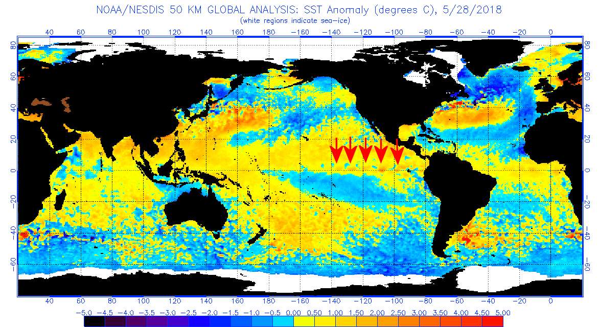
Paul Pukite (@WHUT) says:
” An aircraft’s wingspan is too small to show any differential response to the earth’s Coriolis effect,”
We did an experiment in physics, the one with the guy on a rotatable chair with a spinning bike wheel held by the axles in his hand. The wheel resisted being turned out of the perpendicular and in turn could make the guy spin around on the chair.
Is any of that Coriolis force and would the angle of turn of a plane in a short sharp circle be effected by such forces?
I remember working on train wheels on a North South running train in Darwin where over a long span of times the wheels would wear unevenly necessitating a trim of the metal to realign them which was a Coriolis effect.
Do Dan Hughes and dpy6629 think the Tropical Instability Wave is chaotic? Wikipedia says it has a wavelength of 1100 km. From the image there are 4 wavelengths in 40 degrees longitude, which places the wavelength at 40000km/4*40/360=1111 km. That image from JCH is from a few days ago 5-28-2018, and lo and behold, the TIW is exactly the wavelength as predicted.
Exactly what chaotic process would produce something with this regularity? Seriously, Dan Hughes should be able to answer these kinds of questions as long as he asserts that climate is chaotic.
My assertion Paul is that the effects of turbulence is large in terms of the energy flows in the climate. One cannot model connection without including its effects somehow. What you are talking about here may or not be chaotic but clearly Rossby waves are chaotic in the classical sense.
Please show us the turbulent energy flow on the order of an ocean dipole. You do realize that ocean dipoles are responsible for a significant fraction of the year-to-year climate variability?
dpy,
This may be true in terms of the details, but in terms of the overall state, I would expect this to be mostly wrong. We all probably agree that dynamical processes can, of course, influence the precise state, but the boundary conditions (or, maybe as Ray suggests, the parameters that set these boundary conditions) will be the primary factors that set the equilibrium state and turbulence is very unlikely to strongly impact this.
60. The quality of the large-scale flow simulated in GCMs
https://www.gfdl.noaa.gov/blog_held/60-the-quality-of-the-large-scale-flow-simulated-in-gcms/
“I would also claim that these turbulent midlatitude eddies are in fact easier to simulate than the turbulence in a pipe or wind tunnel in a laboratory. This claim is based on the fact the atmospheric flow on these scales is quasi-two-dimensional. The flow is not actually 2D — the horizontal flow in the upper troposphere is very different from the flow in the lower troposphere for example — but unlike familiar 3D turbulence that cascades energy very rapidly from large to small scales, the atmosphere shares the feature of turbulence in 2D flows in which the energy at large horizontal scales stays on large scales, the natural movement in fact being to even larger scales. In the atmosphere, energy is removed from these large scales where the flow rubs against the surface, transferring energy to the 3D turbulence in the planetary boundary layer and then to scales at which viscous dissipation acts. Because there is a large separation in scale between the large-scale eddies and the little eddies in the boundary layer, this loss of energy can be modeled reasonably well with guidance from detailed observations of boundary layer turbulence. While both numerical weather prediction and climate simulations are difficult, if not for this key distinction in the way that energy moves between scales in 2D and 3D they would be far more difficult if not totally impractical.”
The turbulent cascade is downwards to ever smaller scales.
Turbulence is not the dominant process, z<<x and z<<y
“This may be true in terms of the details, but in terms of the overall state, I would expect this to be mostly wrong.”
Am I wrong or is dpy suggesting that nothing prevents the effects of turbulence from making it cold while the sun is up and warmer at night? And what we are saying is that regardless of the unpredictable local effects of turbulence, there is nothing to suggest that it could disrupt energy balance for extended periods of time. The system will tend toward energy balance as a boundary condition. It will not tend to move away from balance for extended periods.
Steven,
Yes, that would seem – in my view – to be a reasonable summary.
I think someone here watched The Day After Tomorrow w-a-a-a-a-a-a-a-a-y too many times …
https://en.wikipedia.org/wiki/The_Day_After_Tomorrow
“Eventually, a storm system develops in the northern hemisphere, splitting into three superstorms above Canada, Scotland, and Siberia. The gigantic “hurricanes” pull frozen air from the upper troposphere into their center, sending air temperature there below -150 degrees Fahrenheit. The subzero temperatures of the superstorms’ eyes cause flash freezing. Meanwhile, the weather becomes increasingly bad around the world, Tokyo is struck by a giant hail storm and Los Angeles and Hollywood are devastated by a tornado outbreak.”
Chaos Theory predicts that this will happen. Small quasi-2D atmospheric flows (usually called low and high pressure systems) continue to grow in size to reach global proportions. Hurricanes grow to global scale, tornadoes grow to global scales, dust devils grow to global scales. Don’t flush your turlit because it too might reach global proportions.
I’m sort of wondering if Chaos Theory and Turbulence explains our oceans overturning (e. g. the AMOC) or if there are other dominant body forces at work. Or if the ice sheets melt so fast that ocean overturning stops for awhile.
Would we try to explain that as a changing boundary condition or as a product of Chaos Theory and Turbulence?
EFS,
My understanding is that if the AMOC were to stop then it would not simply be a consequence of the chaotic nature of the system. I did read an explanation for this (from Gavin Schmidt, I think) but I can’t quite remember what it was.
and if turbulence could upset energy balance for extended periods we could expect to have seen this in our planets history or the history of all the other planets we observe.
the evidence for the view seems lacking
analogies to cfd, is not exactly evidence about the actual climate
ATTP,
I’m trying to find something that is truly global in scale (e. g. the AMOC appears to fit that bill).
Thermohaline circulation
https://en.wikipedia.org/wiki/Thermohaline_circulation
Shutdown of thermohaline circulation
https://en.wikipedia.org/wiki/Shutdown_of_thermohaline_circulation
Hansen16 suggested this mechanism due to polar ice cap melt accelerating to the point that it overwhelms the associated turbulent overturning mixing structure, or some such.
Here’s a tweet from Gavin suggesting that it’s to do with the difference rates at which the two hemispheres warm. There will be a point at which the density of sub-polar water in the two hemispheres is similar and, hence, the circulation turns off. When they start to differ again, it turns back on.
ATTP,
May 29, 2018! Can’t get much more timely than that tweet. 🙂 I see that Gavin references a new paper. Would that be worthy of a new post?
Multi‐century instability of the Atlantic Meridional Circulation in rapid warming simulations with GISS ModelE2 (paywalled)
https://agupubs.onlinelibrary.wiley.com/doi/abs/10.1029/2017JD027149
If dpy6629 is suggesting that turbulent flow is strong enough that it will overpower the seasonal variation in the global temperature anomaly, I find that hard to accept.
I didn’t make myself clear. By turbulence, I mean small scale fluctuations. For example, wind speed is very noisy at the surface and that’s due to turbulence.
My assertion is simply that the presence of turbulence dramatically changes the overall forces and energy flows. If you compared a flow without turbulence to one with normal levels of turbulence you will see dramatic differences. In CFD we call that laminar flow vs. turbulent flow. There is a huge difference in all aspects of the flow fields. You can see this in how turbulence is modeled, i.e., with eddy viscosity. Roughly a turbulence patch of fluid behaves as if its viscosity is a lot higher than a non-turbulent patch of fluid.
This means that to have any chance at predicting the flow, you must account for turbulence somehow either with eddy viscosity or by some other means.
Counterintuitively, a turbulent boundary layer is more stable in terms of its global properties than a laminar boundary layer. Hard to believe but true. Eddy viscosity (from the turbulence model) is added dissipation that stabilizes things macroscopically.
Just to be clear, turbulence is only one form of chaos in the planetary system as Edward points out. Convection is chaotic at a larger scale level as are Rossby waves. Chaos is the normal natural state of most fluid systems.
Edward, I’ve seen Held’s statement many times. He is talking about Rossby waves. That’s what weather forecasting is all about. What he says explains why weather models have a chance to work. The planetary system has many other phenomena that are very critical to climate such as convection where the turbulence is fully 3D and harder to model.
Let me say one more thing that might help ( or maybe not). The final state of the system is mostly determined by the initial and boundary conditions, even though it can be a sensitive function of these conditions. Turbulence is a critical energy dissipation mechanism that has a large effect on that final state.
dpy,
I’m not sure in what way you think you’re helping. Try reading some of the earlier comments. Repeating things that are wrong isn’t going to make them right.
Well, lets try a thought experiment. If turbulence doesn’t effect the overall flow, why is there a huge literature on it in CFD and why do virtually all real world simulations use turbulence modeling? Its because turbulence is a stabilizing and energy dissipation mechanism that has a strong influence on the overall flow characteristics.
dpy,
I’m on my phone, so will keep thks short. Turbulence almost certainly influences the flow. It almost certainly is, however, not particularly important when it comes to the overall energy balance (I.e. it doesn’t particularly impact the balance between energy coming in and energy going out).
dpy6629 said:
There is no turbulence in large-scale tidal flows. Also, turbulence obviously does not break up the oceanic dipoles. What dramatic difference would you see in a dipole? The closest thing to turbulence is the idea of wave breaking, which occurs at an unsustainable maximum amplitude. And that would tend to diminish the strength of variability anyways.
Consider air in a box at a set temperature. The air is considered a fluid. Obviously this state is best modeled as a statistical mechanical partition of particles following a Maxwell-Boltzmann distribution. Yet, that’s not strictly classified as a chaotic behavior. What’s more, that’s not going to show any spontaneous variability, contrary to what would you are implying for a much larger scale.
Chaos is normally defined as a collective motion, and that is never considered a “normal natural state”. The only way to get a collective motion is by a forcing. Hadley cells are more regular than chaotic and are a combination of Coriolis and convective forces, right?
dpy,
Okay, here’s a longer response. Turbulence clearly impacts flows and how energy is dissipated within the atmosphere. However, in order for it to play a substantial role in influencing the overall energy balance, it would need to impact the flow of energy into, or out of, the system, and it is hard to see how it could do this. These flows are essentially the incoming solar flux, the albedo (how much is reflected), and the greenhouse effect (what fraction of the surface flux is radiated into space).
You mention convection, which does play a key role in the greenhouse effect, through setting the vertical temperature gradient. We can, however, determine the adiabatic gradient from first principles. The actual gradient in the atmosphere doesn’t always match the adiabatic gradient (i.e., the environmental lapse rate can differ from lapse rate). However, this will set the gradient to which we would expect it to tend. If the actual gradient is shallower, we’d expect radiation to heat the lower levels of the atmosphere until the gradient steepens towards this. If it is steeper, it becomes convectively unstable, and the gradient decreases towards this. Therefore, we’d expect this adiabatic gradient (or lapse rate) to be a reasonable approximation for what we’d expect the gradient to typically be.
So, the bottom line is that turbulence, non-linear dynamics, and chaos clearly impacts the details of the flows (weather) but almost certainly do not play a big role in setting the overall energy balance, which is key to setting the typical conditions (climate).
So, if you really think turbulence can substantially impact the typical conditions, you’re going to need to demonstrate this far more convincingly than you have. As I think I’ve said to you before, I would really be interested in you demonstrating that you do understand the basics, because I really don’t think that you do.
dpy6629 said:
In statistical mechanics, the initial conditions (and largely boundary conditions for a macro situations) do not impact the final state. What we have in the climate system is a system that is continuously forced by earth’s rotation, Coriolis effect, solar radiation, and lunisolar gravitation. The notable features of the climate system such as Hadley cells, QBO, tides, etc show no influence on initial conditions, as those have long since damped out by the continuous forcing applied.
A thought experiment is that resistance is a dissipative element in an electrical circuit. If you design a resonant circuit, the resistance will damp the response. Ho hum, resistance exists but it doesn’t impact the intrinsic measure (such as the frequency of resonance or forced response frequency).
To get a state-of-the-art analogy, look at the topologically insulator models of equatorial flow suggested by Delplace and Marston. These are very similar to a Hall effect electrical circuit. There is a notable lack of dissipative element in this model, as the topological boundaries form a robust protection against perturbations. Marston thinks this helps explain ENSO and QBO behavior. And it completely contrasts with a chaotic view of flow behavior. It may be complex, as per wave dispersion, but it’s not chaotic.
I would only include second-order dissipation factors as needed. We still need to understand the first-order factors.
From Drikakis and Lischziner, Aeronautical Journal, July 2002.
“The intuitive nature of turbulence modelling, its strong reliance on calibration and validation and the extreme sensitivity of model performance to seemingly minor variations in modelling details and flow conditions all conspire to make turbulence modelling an especially challenging component of CFD, but one that is crucially important for the correct prediction of complex flows.”
I believe that an example of how turbulence affects the energy coming in and going out is convection. In GCMs recent papers show that the sub grid convection model parameters can have a large effect on model ECS. Turbulent dissipation is critically important to the process of atmospheric convection. The entire convective process is chaotic as well.
dpy,
Not really, no. Energy isn’t convected to space, it’s radiated. Convection plays a role in setting the vertical temperature gradient, which does determine the temperature where energy is radiated to space. However, we can largely determine the expected gradient from first principles.
Large? I realise that how this is parametrised can impact the resulting model climate sensitivity. I’ve seen nothing to indicate that this would result in a likely range for the ECS that is different to what is typically presented (1.5 to 4.5K).
The lapse rate is an adiabatic theory and the atmosphere is not adiabatic. In any case, I agree that to 1st order this theory successfully predicts the lapse rate. So one could say that turbulent mixing is a second order effect.
The problem here is that in estimating what we care about, i.e., ECS, small changes can make a big difference and that’s perhaps a more accurate statement than some of my previous ones.
dpy,
1. There are little indications that these small changes will result in the ECS being wildly different to what we expect.
2. This works both ways. If you think these small changes could lead it to being much smaller than we expect, then you should probably also accept that they could lead to it being much larger.
From Nic Lewis:
“Simulation of convection is another, closely related, major problem area for AOGCMs. Like clouds, convection is a sub-grid scale process that has to be modelled by parameterized approximations. How convection is parameterized in a model has a major impact on its behaviour, including on the cloud and water vapour fields it simulates and how they change with increasing greenhouse gases, and thereby on the model’s ECS. For instance, when the French IPSL modelling group recently improved the clouds and convective parameterization of its main model, the ECS reduced (per AR5 Table 9.5) from 4.1°C to 2.6°C It is also notable that a new German model that, uniquely, simulates convective aggregation – which observational evidence suggests occurs – generates a substantially weaker tropical hot spot than other AOGCMs, as well as having a significantly reduced ECS (~2.2°C vs 2.8°C).36 The simulated convective aggregation changes long-wave cloud feedback from significantly positive to significantly negative (although a good part of this change is cancelled out by a strengthening of positive short-wave cloud feedback).”
That appears entirely consistent with the ECS remaining within the range we expect (1.5K to 4.5K).
I like the way that dpy6629 is being gradually herded into a holding pen, completely oblivious to the fate of his original arguments.
NL would never cherry pick low ECS values now would he. Ba-Ha-Ha-Ha-Ha-Ha- … 😉
Oh, and who knew that NL was a climate science numerical modeler? Not I, that’s for sure.
His climate model is called ECSLT1. Ho-Ho-Ho-Ho-Ho-Ho- … 😦
“The actual range of results is much larger. They are not published because they are not deemed credible.”
I just love a really good conspiracy theory. Please do, tell us more.
I seem to recall asking for peer reviewed citations above, as in walking the walk. I posted a couple myself up thread that essentially say ‘we are actively working on it’ or some such.
Since I already know about turbulent and laminar flows and CFD, we will skip straight to those papers that DY cites here that directly address AOGCM’s/ESM’s turbulence modeling efforts and their outputs.
Ready, set, go …
Who knew that turbulence caused … wait for it … fluid flows! Over a dozen graduate level courses in fluids straight down the proverbial drain, as it were.
dpy,
Possibly, but that works both ways (could be larger, or could be smaller).
ATTP,
“Possibly, but that works both ways (could be larger, or could be smaller).”
That is exactly what I had been thinking when I brought up the AMOC. A bifurcation (tipping) point that leads to an even worse climate change situation.
Yes, it is consistent with the IPCC range. I personally believe however that what you see in the literature just as in the CFD literature are what the modelers consider their more credible results. The actual range of results is much larger. They are not published because they are not deemed credible. However, as Zhao et al point with regard to cloud microphysics parameters, there are often not credible data based constraints to limit these parameters. So, on what basis do you “select” the credible model runs? In estimating the uncertainty, it seems to me you should include all parameters that are consistent with the data. For turbulence modeling that’s been done in a pretty thorough way. There is of course also structural uncertainty.
It’s also worth highlighting what Ed quoted above from Held: “I would also claim that these turbulent midlatitude eddies are in fact easier to simulate than the turbulence in a pipe or wind tunnel in a laboratory. This claim is based on the fact the atmospheric flow on these scales is quasi-two-dimensional. The flow is not actually 2D — the horizontal flow in the upper troposphere is very different from the flow in the lower troposphere for example — but unlike familiar 3D turbulence that cascades energy very rapidly from large to small scales, the atmosphere shares the feature of turbulence in 2D flows in which the energy at large horizontal scales stays on large scales, the natural movement in fact being to even larger scales. In the atmosphere, energy is removed from these large scales where the flow rubs against the surface, transferring energy to the 3D turbulence in the planetary boundary layer and then to scales at which viscous dissipation acts. Because there is a large separation in scale between the large-scale eddies and the little eddies in the boundary layer, this loss of energy can be modeled reasonably well with guidance from detailed observations of boundary layer turbulence. While both numerical weather prediction and climate simulations are difficult, if not for this key distinction in the way that energy moves between scales in 2D and 3D they would be far more difficult if not totally impractical.”
He would not say that if the turbulence in the boundary layer was not critical to the dissipation of energy in the system.
From an APS transcript:
Click to access climate-seminar-transcript.pdf
This may not be science, but it’s important.
From a comment thread at SoD’s:
Search of “GCMs” to see where we’re heading with “GCMs recent papers.” As always, do not miss paulski0’s comments. I’d say Very Tall won the thread, but I might be biased. One could argue that this comment thread was quite dissipative. I blame the ClimateBall meandering. I hope if you get my drift.
[Puts on Donald J Trump MAGA hat]
How can the oceans warm if all that incoming energy drives all of Earth’s circulations which is then eventually dissipated as turbulence?
Maybe it is all that turbulence that is warming the atmosphere and oceans (friction=heat)? Plus all 18TW of mostly FF energy mining, production, and burning.
The Coriolis force is a farce because everyone knows that the Earth is flat.
Why hasn’t the flat Earth stopped rotating? One would think that after ~4.7 billion years (or 6000 years for us YEC) that all that turbulent tidal dissipation and turbulent convective dissipation would have stopped Earth’s rotation. Oh wait, it has stopped rotating or ever even rotating, geocentrism means that the flat Sun rotates around a fixed flat Earth.
[Takes off Donald J Trump MAGA hat]
I actually agree 100% with Held’s statement. The analogy with a wing is good here. Wing lift is essentially a linear function of angle of attack over a pretty broad range. CFD is pretty good at predicting that its linear, in fact linear potential flow predicts this even though its a very simple model. The problem here is that we really care most about the actual value of the lift. Once you start trying to get that right the linear model is useless and you get 100 years of theory and millions of journal papers and person years of research. And then there is drag which is much harder because its so small compared to overall inertial forces.
So, chaos doesn’t mean we can’t predict some things about the system. However, once you get down to quantitative things (and small quantities such as temperature anomaly or drag) its a tremendously hard problem.
And there is a lot of selection bias in the literature on modeling too so uncertainty tends to be understated in some cases dramatically so.
And I should add that to get the lift anywhere near to correct (within 20%) you have to model the turbulence and all the chaos in some way.
It’s pretty clear from palaeoclimate that all this ‘but chaos’ stuff is just rhetoric. Crank up the GHGs and you get a hyperthermal. Crank up NH summer insolation during the Pleistocene and you get an interglacial. Reliably. Repeatably.
Uncertainty in Model Climate Sensitivity Traced to Representations of Cumulus Precipitation Microphysics
It’s worth noting that we’d be delighted if climate science could constrain sensitivity to within 20%.
I think a lot of this comes back to the point I tried to make earlier about how the problems of aeronautical engineering and climate science are fundamentally different in the questions they are trying to answer.
I’ll also reiterate that if someone is an expert in their field and knows that all the other experts are mistaken, commenting on blogs would not be an obvious way to go about putting things right.
Follow Nic Lewis’ example and publish your hypothesis, if you actually have the expertise and want to make an impact on the field.
> The analogy with a wing is good here. […] The problem here is that we really care most about the actual value of the lift.
Many people care about many things. I would care about the possibility that the analogy breaks down before it bears into fruition. The chaotic aspects of climate might not prevent seasons from happening any time soon. The same should apply to estimating a lift. We already have a lift equation, which relies on a lift coefficient:
It is my personal opinion that climate systems evolve at a lower speed than planes, e.g.:
What on Earth, Wind and Fire goes as fast as this bird in stoopid modulz?
VTG, I’m sorry for using the 20% relative error for lift as it is not really analogous. I should have used the drag error which is more analogous. The problem here is that what we care about in climate is a small change in energy fluxes. 3.7 W/m^2 is only a percent or so of total flux at the surface. A more appropriate analogy here is the drag of a wing which is likewise only a few percent of the lift force. Drag percentage errors are much larger and can be up to 100% or even more. A hundred years of work have enabled us to get within 5% for drag, but we use much more fit for purpose tools (steady state models) with massive investments and the problem is vastly easier than the earth system. We have rigorous error estimating tools that enable controlling numerical errors, etc. Our tools take a couple to perhaps 100 core hours so we have run them literally hundreds of millions of times.
I’m not going to try to publish any climate papers anytime soon and I’ve explained this before. I have vastly more interesting fish to fry and a much more attentive and respectful audience than the climate world. I will try to change the reporting of model uncertainty in CFD and that’s a big enough task for any one person.
Climate modelers are actually recently stepping up to the plate a little anyway. There are some recent negative results about sub grid models. It also appears that they are going to be more direct about reporting their tuning efforts. In reality, I think most climate and weather modeler builders already know what I’ve said here. Just as in CFD, it’s those who use the models who perhaps are not fully cognizant of the uncertainty and the literature gives a strongly false positive impression.
JCH, Thanks for that excerpt. That’s from Zhao et al is it not? They did a good job I think.
I linked to it so others, those who want to, can go see where you have gone off the rails.
@-dpy6629
“The problem here is that what we care about in climate is a small change in energy fluxes. 3.7 W/m^2 is only a percent or so of total flux at the surface.”
I am not convinced that invoking sub-grid scale chaotic turbulence to dissipate energy and provide a reduced climate sensitivity is an attractive option.
Regional or local chaotic convection with a high energy flux sounds rather like ‘storm’. Or thunderstorm, tornado, flash-flood, hurricane ?
Might be preferable to have the temperature rise…
But seasonal and diurnal temperature cycles indicate that chaotic dissipation can affect the variance, but not the trend.
Well, JCH, always glad to learn something. 🙂
To look at a reply at SoD related to the above:
“…those who want policy action can enlist the support of many more people for policies which are proportionate to credible lower bound estimates for warming, and its consequences, than for policies proportionate to worst case estimates of warming.”
Assume all us reformed deplorables but still lukewarm after all these years want the lower values. The higher values break things. We will not follow that far. The break means, that is why the marketing fails. This is simply middle positioning of the product. If 4.5 C appeals to you, the marketing is different. What does a survivalist do? The higher threat appeals to them, and they buy a lot of stuff. Most of the rest just vote Republican and pay their taxes while not moving to Montana.
dpy6629 complains about incorrect computational gridding leading to numerical errors.
No doubt that can happen, and if a calculation may take hours to do and then you have to multiply that by a number of runs to perform parametric fitting, that will eat up an incredible amount of time.
The solution to this is to do the computations analytically, focusing on a specific climate behavior. With an analytical formulation, the computation is miniscule and one can run optimizing solvers to fit to the data.
Voila, no worries about error propagation and it’s fast and cheap. Of course, some think this is a pipe dream.
@-W
“What on Earth, Wind and Fire goes as fast as this bird in stoopid modulz?”
Don’t know about stoopid modulz, but the plasma ball stratospheric lighting above thunderstorms, sprites, are said to reach 10% of light-speed.
(grin)
Yes Paul, I like simple analytic models too. Just wish there was more work being done on them. People tend to just run very complex codes with “more physics” because its easy to do.
Well Willard the Reynolds number also depends on the size of the object. I’ll give you a formula later. In any case lower Reynolds number flows are actually harder.
http://rsta.royalsocietypublishing.org/content/367/1890/815
Vintage 2009. That’s nine years ago.
I’ve thought in more detail about the convection issue. The role of turbulence seems to be to highly dependent on the convective strength.
If the convection is weak, vertical velocities are small the the shear layers will stay laminar. In this circumstance adiabatic theory is not a bad approximation.
Once vertical velocity passes a threshold, the shear layers become turbulent and contribute to horizontal mixing (non adiabatic).
In strong convection, the whole parcel of air is very turbulent as in a thunderstorm. The lapse rate theory seems to me to be very wrong in this case and turbulence dominates.
So what is the “average”behavior? I have no real thoughts on that except that we know now that convective modeling can have a strong influence on ECS in a GCM. Aggregation of convection seems to lower ECS, and aggregation happens in nature. This is of course complicated by clouds and precipitation and we know clouds have a strong effect on ECS. In the absence of strong data constraints, I find it hard to believe that a simple sub grid model on a 100 km box can possibly do an adequate job of “averaging” this complex behavior. But I’d like to see any evidence either way.
The same is true of the planetary boundary layer. If wind velocity is very low, turbulence is irrelevant. But as everyone knows from direct observation if the wind is even O(5 mph) turbulence is quite prominent and GCMer’s know they must model it. Whether they do an adequate job is open to question but it has a large effect in dissipating Rossby waves.
Where I do question Held’s assertion about Rossby waves and 2D flow. We know from observation that the atmosphere is very turbulent at all altitudes. Much of this might be wind shear but it is clearly fully developed 3D turbulence. It will play a significant role in getting dissipation levels well enough to propagate the waves too far.
One thing to note Willard in your figure is that as Reynolds number increases the number of mesh points grows dramatically. Adaptivity is probably an asset in climate modeling but there is a big hurdle there to overcome. Also the flow features are a strong function Reynolds’ number. The higher Reynolds’ number is probably significantly turbulent. This demonstrates how important viscous effects are in modeling even very gross global properties. And yes turbulence is a very important component of viscous effects.
@-dpy6629
” In the absence of strong data constraints, I find it hard to believe that a simple sub grid model on a 100 km box can possibly do an adequate job of “averaging” this complex behavior. But I’d like to see any evidence either way.”
The evidence for strong data constraints lies in the diurnal and seasonal cycles.
Your ‘magical’ turbulence is swamped by the change in forcing, it does not make night hotter than day, or summer colder than winter.
It affects variance, not trend.
“it does not make night hotter than day, or summer colder than winter.”
ur welcome
Except Izen that recent papers shows that modeling of turbulent processes can affect the trend too. Zhao et al given above by JCH is an example. But I’m not saying anything controversial here.
and turbulence can obviously violate energy balance over centrury timescales?
the output from the sun could go to zero and turbulence could keep us warm.
or not?
@-dpy6629
” But I’m not saying anything controversial here.”
That is because you are not saying much of anything.
You are hand-waving towards turbulence as a causal explanation for … what? beyond local weather it is difficult to see what influence you think it could have.
Could you detail or cite the evidence for chaotic processes in the climate shaping the trend that is caused by a change in forcing, like the CO2 rise, or seasonal changes, or diurnal ranges ?
Could you describe what evidence would cause you to regard your ideas on the influence of CFD on climate to be wrong, or at least in order of serious reconsideration ?
The Zhao paper, and the Nick Lewis comment are not about actual trends, the modulz can produce close versions of the observed climate trend with different amounts of variance depending on the details of how some aspects are parametised. That affects the climate sensitivity you can calculate using EBMs from models, (and observations) making that method uncertain.
In neither the modilz nor observations show CFD affecting the underlying trend.
Unless you can cite credible research that shows otherwise ??
@-SM
“ur welcome”
Thank you. You were the first to point out the extreme lack of evidence for macro effects from turbulence in the historical climate record. Then Willard tried with Held’s observation about the linearity of the system, as evidenced by seasonal patterns. A point first accepted, then rejected in a subsequent post by dyp6629.
It would be madness to expect that an argument already ignored twice would have any impact if made again. But I stole it anyway.
(Grin)
dpy,
What trend? As izen has already said, it can impact climate sensitivity and, hence, how much we would warm for a given radiative perturbation. However, there are no real indications that it will result in a climate sensitivity wildly different to what we expect. On the other hand, one could argue that it implies a greater uncertainty. However, given how much we’ve already warmed, it seems really unlikely that ECS can be less than 1.5K, so if you do want to increase the uncertainty, it might imply a greater chance of a high ECS, rather than a greater chance of low one.
“What trend?”
Yeah, what ‘so called’ recent papers?
3rd time I’ve had to ask for citations. If you really want to be taken seriously, then post some relevant climate science numerical modeling papers (related to their turbulence formulation(s)).
dpy6629 said:
Maybe I don’t understand turbulence, but I can swear that air moving collectively at several hundred miles per hour in a jet stream is not turbulent. The QBO in fact may not even be considered a conventional wave, as it’s wavenumber is zero. It has effectively an infinite wavelength as it wraps around the equator. Yet it’s still a wave as it does have a frequency, and is probably a perfect example of laminar flow.
But to egg you on, you must understand what causes the QBO to reverse directions? C’mon, with all your experience with wind-tunnels, it should be peanuts to explain this.
Yet here we find you, again and again, hour after hour. I’m sure you can see how this seems a little, well, inconsistent to a casual observer.
Ah, the Cartman gambit. Often seems to be a strong driving force for contrarianism.
vtg,
It is interesting that someone who seems to show very little respect for others, objects to the lack of respect shown towards them.
Fluid motions in the atmosphere and oceans on Earth’s surface are not the only situations in which the Coriolis effect is encountered by engineers. Raleigh-Benard convection is usually demonstrated by rotating experimental rigs of various geometry and rotating parts, for example. Fluid motions inside engineered equipment, like a pipe, say, occur under all kinds of non-stationary rotating and accelerating frames, power plants on ships, for example. Getting the geometric details of the locations and flow directions relative to the power plant and inertial frames generally requires a whole nother level of geometric description information. And, of course, it matters where the system is located on the planet. I ‘m certain that aeronautical engineers account for the effects of non-stationary rotating and accelerating frames on some motions and loads of aircraft. Equally certain that the effects are accounted for in the power plants here, too.
As fun homework problems we are sometimes asked which side of the banks of rivers have a higher potential for erosion for rivers that flow N-to-S, S-to-N, E-to-W, or W-to-E. And, how do bends in the river path modify this behavior. The forces and potential for wear on railroad tracks is another application.
What happened to my picture of an aeroplane? Try it this way:
aeroplane
From later in the 20th century. Seems like hydrostatic models remain Ill-Posed Initial-Boundary Value Problems.
G.L.Browning, W.R.Holland, H.-O.Kreiss, and S.J.Worley (1989). An accurate hyperbolic system for approximately hydrostatic and incompressible oceanographic flows, Dynamics of Atmospheres and Oceans vol. 14, pp. 303-332. https://doi.org/10.1016/0377-0265(89)90066-3.
Abstract
It is well known that severe restrictions on accuracy and stability arise when using a numerical model based on the Eulerian equations to compute the low frequency motions of physical oceanography. The loss of accuracy is due to the extreme skewness of the system. Although the system can be transformed to symmetric hyperbolic form, the diagonal transformation matrix contains factors that produce mathematical estimates indicating loss of accuracy and these estimates are verified in practice. The stability restriction is just a result of the multiple timescales present in the system, i.e. the presence of Rossby, gravity, and sound waves. Three alternatives to overcome these restrictions are discussed.
The first two alternatives are the primitive and quasi-geostrophic equations. Although models based on these systems alleviate some of the restrictions of the Eulerian model, they operate under a new set of limitations. The primitive equation model requires more resolution than a quasi-geostrophic model to obtain the same degree of numerical accuracy and is ill-posed for the initial-boundary value problem. Although the quasi-geostrophic equations are accurate to the order of the Rossby number, there are cases when this error is of the order of 10%. Reducing the error in these cases, e.g. by using the balance equations, requires a considerable increase in the computational complexity of the system. The quasi-geostrophic equations also cannot be used in the equatorial region and any improvements which would allow them to be used there would result in a computationally inefficient system.
The third alternative is to slow down the gravity and sound waves by decreasing the size of the appropriate terms in the equations. Although the resulting approximate system alleviates the severe accuracy requirement, the stability requirement may still be unacceptable. By using the reduced system derived from the approximate system, a system which has many desirable properties is obtained. The resolution requirements for a model based on the reduced system are the same as those of the quasi-geostrophic model, i.e. less than for a model based on the primitive equations. Because the reduced system is the proper mathematical limit of a hyperbolic system, a wide range of boundary conditions can be chosen so that the resulting initial-boundary value problem is well posed. The reduced system analytically describes the low-frequency solutions to two digits of accuracy (even when the Rossby number is O(0.1)), yet only requires the solution of a linear, constant coefficient, three-dimensional elliptic equation. Finally, the reduced system is applicable in the equatorial region.
Here we go. From early in the 21st century:
In December 2013, early in the 21st century, Professor Dargan M. W. Frierson, University of Washington, Department of Atmospheric Sciences, in this presentation summarized the the status of the GCMs that supplied results for CMIP3:
Of 24 models in the CMIP3 archive (models used for IPCC AR4): 1 was non-hydrostatic (Had-GEM)
So, early in the 21st century, 23 of the 24 GCMs are all Ill-Posed Initial-Boundary Value Problem models.
Dan, it’s painfully obvious you don’t understand the subject.
Googling until you find a hit you think matches your notions does not constitute understanding.
Steve, Of course energy is always conserved. Turbulence changes the rate at which inertial energy is dissipated into thermal energy.
The TCR will affect the rate of temperature increase. The TCR can be engineered in a GCM over a broad range by turbulent process parameterizations. Zhao shows that.
Ah GL Browning again.
Related.
VTG, My observation is that the CFD community is less political. Generally most people are honest and direct and often very intelligent. Learning is a lifelong pursuit and here I learned something about the lapse rate theory and turbulence. Thanks to ATTP. Thanks for interacting on that.
Steve, I think Browning is making a different point but I believe its correct. Basically Gerry is saying that the hydrostatic approximation used in GCM’s is a bad choice. I think it was Browning’s thesis advisor, the name escapes me, was the one who came up with an critical improvement for GCM’s at NCAR for filtering out sound waves which were destroying the accuracy of their results.
dpy,
1. I don’t think this is true to the extent that we would expect it to substantially change the likely range.
2. My understanding is that this is mostly related to cloud feedbacks. There are others lines of evidence suggesting that cloud feedbacks are probably positive.
3. If cloud feedbacks are positive, the the ECS is probably greater than 2K.
4. The TCR-to-ECS ratio is probably between 0.6 and 0.8. If the ECS is > 2K, then the TCR is probably > 1.2K.
5. We’re back to a range comparable to that presented by the IPCC.
A maxim I would suggest equally applies to all scientific disciplines.
VTG, Some are more honest than others. There are some people in CFD who are not honest too. Generally though those in CFD don’t have a political axe to grind. For example recent scientific evidence shows that psychology is worse than other disciplines in terms of replicatability.
With regard to the IPCC range for ECS. My belief is that the uncertainty in the GCM estimates is understated due to selection bias.
Lack of replicability and lack of honesty are not synonymous.
Resorting to attacking an entire discipline as dishonest makes you appear to lack the ability to make technical arguments.
Dan Hughes said:
Yes, and it is one of those behaviors that scales according to the radius of the object. There will only be a significant Coriolis effect for large scale systems on Earth because of the differential forces required on the inside (i.e. equator) and outside edge. (Try stumping the chump about directions that toilets flush north and south of the equator. Admit that I’ve been fooled by this too)
dpy6629 says:
Lapse rate models are steady-state results, so the rate there does not matter. Try again.
Amazing how the mechanics of the entire universe can be explained by the failure of some studies to replicate the findings of previous studies (and political bias on the left, of course).
Dan Hughes quotes a paper:
Aha, the equatorial regions are the prime areas for simplification of the primitive equations. In both oceanic and atmospheric regimes, the Coriolis effect exactly cancels here and analytical results are possible. No wonder they can’t use quasi-geostrophic equations, because there is nothing to balance out!
> My observation is that the CFD community is less political.
Yet here you are. For once it was going well. Why does it need to be turned into technical comments? Speaking of more interesting fish to fry:
Not sure how we can both claim that uncertainty is bigger and climate sensitivity more constrained, yet here we are.
VTG, It would be helpful if you didn’t put words in my mouth. I never said an entire field was dishonest nor do I believe it in any case.
dpy,
That’s pretty much how I interpret what you say. If you don’t like that interpretation, maybe try harder to not make is seem that you regard an entire field as dishonest. And, fwiw, telling us that it isn’t what you think, while saying things that make it appear that it is what you think is not a convincing way to do so.
Well Willard, There is no contradiction. My claim is that GCM’s are not really valid scientific evidence about ECS. That leaves us with other lines of evidence. I don’t know really how well constrained ECS is by those lines of evidence even though I’ve not seen any detailed scientific critique of Lewis’ work. That work has weaknesses but has the virtue that energy is conserved in the real world. What worries me a bit is that the method might be numerically sensitive to the forcing estimates and indeed Nic has said as much.
> I never said an entire field was dishonest nor do I believe it in any case.
Here’s what you said:
Very Tall’s “Resorting to attacking an entire discipline as dishonest makes you appear to lack the ability to make technical arguments” looks like a fair paraphrase of what you’re insinuating.
I suggest that from now on, you keep your technical comments about honesty to Judy’s or elsewhere.
The comment threads have been moderating themselves for more than a month now. I’d like to keep it that way, if you don’t mind.
“Insinuation” is a tenuous thread of textual criticism to fall back on.
You’ve been attacking the GCMs community for more than a decade, DavidP. This time, it’s by comparing it to the CFD community, which you characterize as less political, more intelligent, and more honest. The logical transformations to turn what you said into an attack such as described by Very Tall (whom did not put any word into your mouth, if you want to get technical) are pretty straightforward.
Now, I really suggest you return to Reynold numbers and stuff.
dpy6629 wrote “Generally though those in CFD don’t have a political axe to grind”
I think it is more that those working on CFD are not attacked/insulted/misrepresented by those with a political axe to grind. It is a career limiting move to allow politics to interfere with your scientific judgement, and I suspect that most climatologists are perfectly well aware of that.
Actually, maybe we can rein this in. By normal climate blog standards, this discussion has been reasonable.
That’s good to hear, and sorry that I misinterpreted your remark.
It would be helpful perhaps in future not to refer to “honesty” unless making a direct claim. Otherwise such misinterpretations are, as we see here, perhaps more easily misinterpreted than not!
dpy,
Nic’s work is also very sensitive to the choice of present and historic periods chosen and also the temperature data set used.
However, I would ask a broader question about TCS/ECS. If TCS/ECS is low what does that mean for climate change impacts and what is your evidence? I ask as an engineer involved in designing critical infrastructure, often with a design life of 100 plus years.
HH, I actually think Nic looked at quite a few base and current periods and his claim is that its not very sensitive to that.
I am not going to get involved in “impacts.” This is an area where GCM dependence is rife and statistics is questionable in my view. We know sea level is going to keep rising so that’s an area we can address with policy. Other than that I’ll leave the impacts to you.
@-dpy6629
” My claim is that GCM’s are not really valid scientific evidence about ECS. ”
How do you measure ‘really valid scientific evidence’ ?
Remember, all modulz are wrong, some are useful.!
@-“That leaves us with other lines of evidence.”
Paleo, volcanic, and seasonal events are the obvious candidates. Observational and proxy data can give a valid estimate of the change in forcing and the change in temperature.
Despite the GCM’s lack of ‘validity’ they turn out to be pretty good at simulating those changes. They may get CFD or cloud/precipitation wrong, but the results are still useful, even if not ‘valid’.
EBM have the disadvantage of short timescale observations (large variance) and the small size and uncertainty of the forcings. Plus the simple modluz used by EBMs of atmospheric loss and rate of ocean absorption, carry all the problems of validity you are claiming apply to GCMs.
In spades.
[Snip. Next time, DavidP, I won’t take the time to snip. -W]
There are some obvious steps that can be taken in CFD and climate/weather modeling that will improve the quality of the science. The CFD literature is strongly biased in the positive direction, i.e., it gives a false impression about how accurate CFD really is. The cure for that is preregistration of all CFD validation exercises. You have to state what you are going to run, what the parameters are, what the grids are going to be and what hypotheses you are testing. Similarly for GCM runs. This prevents what I call “CFD hacking.” You simply run the code trying various things until you get what you think is a credible result.
Another big step forward would be to employ statisticians on all studies that use statistics. CFD era often roll their own statistics and that inevitably invites skepticism.
In medicine both of these steps are starting to take hold and there is evidence that both work to improve the science.
ATTP sez:
And exhibited by palaeoclimate. Well, to be fair, palaeoclimate behaviour suggests that a high-ish central estimate may be closer to reality.
dpy,
What you’re suggesting doesn’t really work in some areas of science (in my view, at least). There are reasons why you would want to pre-register your studies in some areas of science (medicine). You don’t want people to get a negative result and simply not report it. Why would you do it in CFD? If you code fails a test, then you would fix it. Why would you waste people’s time writing a paper to point out that your code failed a test. If your code produces a result that is clearly not physically plausible, why would you publish a paper pointing out that your code produce a physically implausible result?
Of course, I’m assuming here that people will be honest. If a code fails a standard test, you wouldn’t simply carry on and ignore that it failed a test; you would fix the code.
Willard, The focus of my early criticism was that GCM’s often use quite old numerical methods some of which have known flaws. That is still true. I’m no longer so sure however that big gains can be made by introducing more modern methods. I realized about 4 years ago based on how CFD was going the time accurate eddy resolving route that the real issue is theoretical, what is the attractor like? That’s what we really need to address.
What I see now is that all CFD has these very big theoretical issues that seem to always go unaddressed. We direct huge resources to “running the code” and very little to the fundamental math and science. That’s a universal problem.
dpy2966 said:
Contrast CFD to the field of GFD (Geophysical Fluid Dynamics), which takes in to account the planetary scale of the physics. A good primer is:
“Geophysical fluid dynamics: whence, whither and why?” by Geoffrey K. Vallis
http://rspa.royalsocietypublishing.org/content/472/2192/20160140
Interesting comment by Vallis that I have been mulling over :
“The geosciences in general deal with complex interacting systems and in some ways resemble condensed matter physics”
Agree with this, because as Vallis continues “(in condensed-matter physics) we seek explanations of phenomena at a higher level than simply directly calculating the interactions of all the constituent parts. That is, we try to develop theories or make simple models of the behaviour of the system as a whole.”
It is indeed very rare that you have examples in condensed-matter physics whereby a full dynamical simulation is needed to extract the salient characteristics or behavior of the phenomena under study. To think that detailed simulations are also required for large-scale climate behaviors would make that unique. Yet Vallis also claims that: ” Such simulations, as manifested, for example, in complicated general circulation models, have in some ways been extremely successful and one may reasonably now ask whether understanding a complex geophysical system is necessary for predicting it.”
That is quite an assertion — that one does not need to understand the physics to predict it.
[If you can’t keep your technical comments to technicalities, it might be best you go play ClimateBall elsewhere, DavidY. -W]
@-dpy6629
“In medicine both of these steps are starting to take hold and there is evidence that both work to improve the science.”
In medicine those steps are specifically targeted at research that is concerned with APPLICATIONS of discoveries made.
It is concerned with regulation of the ‘D’ bit of R&D. Nobody would suggest applying it to the research bleeding edge of the field, the expansion of understanding, only to the commercial developments that might be derived from it.
There is no way to register in advance the previously unknown properties of new active organic molecules you intend to discover. Or what methodology you will restrict yourself to using, when ongoing results may indicate more fruitful lines of inquiry.
No more talk about honesty or any related concept, pretty please with sugar on it.
I know very well one of the senior organizers of the first drag prediction workshop. This was a test case that was carefully documented and given to everyone to run in their code without any knowledge of the “right” result. Testing came after the cfd. This organizer said everyone was quite surprised at how scattered the results were. That’s strong evidence that not just the literature was biased but that people had fooled themselves. They had fallen into the idea that ATTP talked about that “if the code has a problem, you fix the problem.” Well if it has bug you fix the bug. But sensitivity to inputs is a feature not a bug.
Actually the CMIP series and these AIAA workshops are helpful and a step forward. The problem with the drag prediction series is that they gradually made the problem easier and narrowed the range of how you could run your code until they got a more palatable result.
You can ignore palaeoclimate David, but it will still be there in the morning 🙂
The snipped comment I think was just about uncertainty in CFD and how it is much larger than most people believe. This is a cultural problem in that there are cultural beliefs about nature and science that are dominant and shape the literature. People are naturally optimistic about their work.
In any case, if you allow people to select their “best” runs, you introduce a bias.
dpy,
I’m not suggesting *allowing* people to keep their best runs. If people run a suite of simulations, they should report on *all* of their runs. However, if they discover some fundamental flaw that needs to be fixed, there is not much point in writing a paper pointing out that you found an error in your code.
I agree with that last formulation.
Uncertainty and Error in CFD Simulations
https://www.grc.nasa.gov/www/wind/valid/tutorial/errors.html
Here’s the goal. Fix the thing.
It may help to analyze the CFD system. Me, I think fluids are just a denser form of the atmosphere, there are commonalities. I see lack of knowledge and round off errors. The second is grid size limit. I think it’s agreed it would be nice to have 100 times the computing power and to say that backwards, we are throwing out 2 significant digits to save time and money, or we are too computer poor to know.
So the work is in a background of these two problems. Lack of knowledge can be summed as clouds but more importantly long term cloud records and many long term attributes of the climate, further boxing us into the short term. So the work happens with these limits and is defined by them.
Can’t do anything about old data we don’t have while I recognize some work is done in that arena. We can buy more computing or lower the cost of computing. It’s agreed that clouds are a problem. But that problem is worked around and not attacked. ARGO started. We need to somehow have adequate cloud data. Matching the surface temperatures results by the models is one thing. Tying out the clouds would show an important temperature control process.
If the CFD tells you the plane will end up in a deep stall, do you fly the test vehicle to that point in the envelop without a stall parachute? and argue that CFD is no good because uncertainty?
Ragnaar said:
No use trying to think through it at your level. Start with the primitive equations here:
https://en.wikipedia.org/wiki/Primitive_equations
Initial Conditions matter.
Working Group I, IPCC AR5 2013
Flato, G., J. Marotzke, B. Abiodun, P. Braconnot, S.C. Chou, W. Collins, P. Cox, F. Driouech, S. Emori, V. Eyring, C. Forest, P. Gleckler, E. Guilyardi, C. Jakob, V. Kattsov, C. Reason and M. Rummukainen, 2013: Evaluation of Climate Models. In: Climate Change 2013: The Physical Science Basis. Contribution of Working Group I to the Fifth Assessment Report of the Intergovernmental Panel on Climate Change [Stocker, T.F., D. Qin, G.-K. Plattner, M. Tignor, S.K. Allen, J. Boschung, A. Nauels, Y. Xia, V. Bex and P.M. Midgley (eds.)]. Cambridge University Press, Cambridge, United Kingdom and New York, NY, USA.
Section 9.2.1.4 says:
The atmospheric component of climate models can be integrated as a weather prediction model if initialized appropriately (Phillips et al., 2004). This allows testing parameterized sub-grid scale processes without the complication of feedbacks substantially altering the underlying state of the atmosphere.
The application of these techniques since the AR4 has led to some new insights. For example, many of the systematic errors in the modelled climate develop within a few days of simulation, highlighting the important role of fast, parameterized processes (Klein et al., 2006; Boyle et al., 2008; Xie et al., 2012). Errors in cloud properties for example were shown to be present within a few days in a forecast in at least some models (Williams and Brooks, 2008), although this was not the case in another model (Boyle and Klein, 2010; Zhang et al., 2010b). Other studies have highlighted the advantage of such methodologies for the detailed evaluation of model processes using observations that are available only for limited locations and times (Williamson and Olson, 2007; Bodas-Salcedo et al., 2008; Xie et al., 2008; Hannay et al., 2009; Boyle and Klein, 2010), an approach that is difficult to apply to long-term climate simulations.
Literature cited:
Klein, S. A., X. Jiang, J. Boyle, S. Malyshev, and S. Xie, 2006: Diagnosis of the summertime warm and dry bias over the U.S. Southern Great Plains in the GFDL climate model using a weather forecasting approach. Geophys. Res. Lett., 33, L18805.
https://agupubs.onlinelibrary.wiley.com/doi/pdf/10.1029/2006GL027567
Boyle, J., S. Klein, G. Zhang, S. Xie, and X. Wei, 2008: Climate Model Forecast Experiments for TOGA COARE. Mon. Weather Rev., 136, 808–832.
https://journals.ametsoc.org/doi/pdf/10.1175/2007MWR2145.1
Xie, S., H.-Y. Ma, J. S. Boyle, S. A. Klein, and Y. Zhang, 2012: On the correspondence between short- and long- timescale systematic errors in CAM4/CAM5 for the years of tropical convection. J. Clim., 25, 7937–7955.
https://journals.ametsoc.org/doi/pdf/10.1175/JCLI-D-12-00134.1
Williams, K. D., and M. E. Brooks, 2008: Initial tendencies of cloud regimes in the Met Office unified model. J. Clim., 21, 833–840.
https://journals.ametsoc.org/doi/pdf/10.1175/2007JCLI1900.1
Boyle, J., and S. A. Klein, 2010: Impact of horizontal resolution on climate model forecasts of tropical precipitation and diabatic heating for the TWP-ICE period. J. Geophys. Res., 115, D23113.
https://agupubs.onlinelibrary.wiley.com/doi/pdf/10.1029/2010JD014262
Zhang, Y., S. A. Klein, J. Boyle, and G. G. Mace, 2010b: Evaluation of tropical cloud and precipitation statistics of Community Atmosphere Model version 3 using CloudSat and CALIPSO data. J. Geophys. Res., 115, D12205.
https://agupubs.onlinelibrary.wiley.com/doi/epdf/10.1029/2009JD012006
Williamson, D. L., and J. G. Olson, 2007: A comparison of forecast errors in CAM2 and CAM3 at the ARM Southern Great Plains site. J. Clim., 20, 4572–4585.
https://journals.ametsoc.org/doi/pdf/10.1175/JCLI4267.1
Bodas-Salcedo, A., M. Webb, M. Brooks, M. Ringer, K. Williams, S. Milton, and D. Wilson, 2008: Evaluating cloud systems in the Met Office global forecast model using simulated CloudSat radar reflectivities. J. Geophys. Res. Atmos., 113, D00A13.
https://agupubs.onlinelibrary.wiley.com/doi/pdf/10.1029/2007JD009620
Xie, S., J. Boyle, S. A. Klein, X. Liu, and S. Ghan, 2008: Simulations of Arctic mixed-phase clouds in forecasts with CAM3 and AM2 for M-PACE. J. Geophys. Res., 113, D04211.
https://agupubs.onlinelibrary.wiley.com/doi/epdf/10.1029/2007JD009225
Hannay, C., et al., 2009: Evaluation of Forecasted Southeast Pacific Stratocumulus in the NCAR, GFDL, and ECMWF Models. J. Clim., 22, 2871–2889.
https://journals.ametsoc.org/doi/pdf/10.1175/2008JCLI2479.1
Boyle, J., and S. A. Klein, 2010: Impact of horizontal resolution on climate model forecasts of tropical precipitation and diabatic heating for the TWP-ICE period. J. Geophys. Res., 115, D23113.
https://agupubs.onlinelibrary.wiley.com/doi/pdf/10.1029/2010JD014262
Dan,
That appears to be suggesting that you can test models in that way, it doesn’t mean that somehow the typical climate state depends on the initial conditions. Having said that, of course the initial conditions can matter (as has already been pointed out). The key point, though, is that the typical climate state depends more on the parameters that define the boundary conditions, than on the initial conditions (although the latter will influence the actual path followed).
Willard quoting Isaac Held, a grad of U of Minnesota:
That is essentially what DH and DPY are missing with respect to the big picture. For the global temperature anomaly, the seasonal cycle is always filtered out because that is well understood. Besides the seasonal forcing, the other clear forcings to consider are the aerosol forcings, which can include volcanic and CO2, the gravitational tidal forcings, and the slight second-order changes in TSI. The most obvious and most significant contributor to the erratic year-to-year fluctuation is the ENSO signal, which can be understood to derive from a tidal forced response to the system. The challenge there has always been to synchronize the lunisolar tidal cycle, which is roughly 372 years in its repeat period, to what is observed in the ENSO cycle. This challenge is more in the realm of geophysicists, satellite engineers, and astrophysicists who need to be able to calculate the orbital ephemerides precisely for other applications. Once one does this and applies it as a guided (not initial) forcing to the Navier-Stokes primitive equations for the equatorial ENSO, the dispersion solution result is striking in its ability to match the data. Paraphrasing what Isaac Held is saying, a primarily linear forced response is the rule for the climate system, but which is contrary to the chaotic response that DH and DPY are hoping for.

Paul, Held is right in that the integrated response can be linear. The problem here is that this observation is not very useful. To be useful you need to know the slope and the value. To find these, you must model turbulence and other chaotic process which effect the slope and the value in some cases a lot. That’s why Held’s group’s GCM includes turbulence modeling in the boundary layer and models of convection and precipitation. Bear in mind that Rossby waves are chaotic too so the chaos is at all scales in the earth system. You must model Rossby waves in a GCM to have any chance of usefulness.
In reality many large changes in climate in the past have happened while integrated forcing remained constant. The distribution of the forcing matters a lot. As I understand it the ice age cycles were caused by changes in local insolation while the total integrated forcing remained constant. The feedback response was nonlinear and had mostly to do with things like ice albedo and dust.
dpy,
You’re missing the point. That the response is *roughly* linear means that we don’t expect massive surprises because of the non-linear nature of the underlying system.
This is rather confused. Yes, the glacial cycles appear to be triggered by large changes in solar insolation at high northern latitudes, but with little change in the overal solar forcing. The resulting changes in albedo (ice sheets) and CO2 (through ocean outgassing/uptake) are what actually drive the change in global surface temperature. If, however, you treat these changes as forcings, rather than feedbacks, you get back to a *roughly* linear response that also allows us to estimate the ECS. The result is an ECS of about 3K +- 1K.
In fact, this is kind of the key point. Yes, the trigger for the glacial cycles might have been associated with a change in the distribution of the solar forcing, but little change in overall forcing, but this produced a change in the boundary conditions (or the parameters that determine the boundary conditions) that then lead to the change in global temperature and the move from a glacial to an inter-glacial (or vice versa). You can’t get this kind of change simply through some internally-driven process (i.e., without also changing one of the boundary conditions).
The problem here ATTP with your explanation is that the ice ages were largely the result of nonlinear feedbacks. To “treat” them as forcings is stretching the language.
The point about the linearity statement is that its of little practical value. Whether we expect nonlinear “surprises” is not very useful in my view. In any case, there are nonlinear surprises that happen rather frequently. That’s why it took so long to figure out the ice ages. It was a complex and subtle process.
Just like in aerodynamics you need to know the slope and value and for that you need either test data or complex CFD where you take account of turbulence and other chaotic processes.
dpy,
You still miss the point. Why did we globally warm/cool during the glacial cycles? It was mostly because of changes in albedo and changes in atmospheric CO2/CH4. If we express these changes as W/m^2, what was the resulting change in temperature. It was about 0.75 +- 0.25 K/W/m^2. What does that imply about how much we would warm if we double atmospheric CO2? Since that produces a change in forcing of 3.7W/m^2, it implies a warming of about 3 +- 1 K.
You’re the one arguing for non-linear surprises. What’s being pointed out is that if you quantify this in terms of changes in forcing, then we expect the response to (on average) depend linearly on this change in forcing. If non-linear surprises happened rather frequently, we’d probably have seen some rather strange seasons. We don’t really. It’s not exactly the same every year, but July is typically warmer than December in the Northern Hemisphere.
dpy6629 said:
Yes, for every order of a differential equation, an additional initial condition is required. So, for a 2nd-order DiffEq, you need f(0) and df/dt(0). Everyone who has taken classes in advanced differential calculus knows this. But what engineers understand in their day-to-day lives is that the forced response is often every bit as important as the natural response — this is because the initial conditions are often completely damped out or subsumed by the forced response to a continuous input.
Do you understand this fundamental idea, dpy66629? Just to be sure, I will keep on asking this question until I get a response.
I understand the point about forcings ATTP. I’m saying that is of little practical value without understanding the very important role of nonlinear feedbacks and chaotic processes and their strong effect on the value and the slope of the response to forcings. In any case, adhering to proper definitions is important to getting anywhere in any discussion. I think we need to keep clear the distinction between forcings and feedbacks, a point you have made many times in the past.
I’m not sure I know if there will be surprises and I’m not arguing for or against it. I’m just saying they happen all the time in aerodynamics where you never know really where nonlinearity will kick in and destroy the “linear” range.
Yes Paul I understand that the initial conditions can get damped out.
I also know that recent research shows that initial conditions and parameters of the model can make a huge difference in the results of RANS calculations. There are multiple solutions, pseudo-solutions too. People are finding that its really hard to get fully consistent results even in the linear region. This is new research but it shows that our naive model of RANS was wrong. It doesn’t behave like a simple 1D ODE IBVP.
dpy,
Sigh. It’s expected to be roughly linear, unless we go ahead and produce a very large change in forcing. If you dispute this, you really should do more than simply wave your hands to non-linear feedbacks and chaos.
I am sticking to the proper definitions.
You’re arguing for non-linear feedbacks, and that non-linear responses are important. Can’t you at least acknowledge what you’re doing?
You also haven’t demonstrated that these possible non-linear responses are probably important in this context. Those who happen to have expertise in this topic explicitly say that we expect the response to be *roughly* linear. If the response was highly non-linear then we would probably have seen evidence for this. This doesn’t mean non-linearities can’t emerge, simply that they are unlikely (again, unless we go ahead and produce a large change in forcing, in which case all bets are probably off).
I like that the best evidence Dan Hughes can provide for initial conditions being important in GCMs is that you have to set initial conditions carefully when trying to simulate weather (for calibration purposes).
Weather: it isn’t climate. If only the debate could rise beyond that level.
It’s like he just searched through AR5 for ‘initial conditions’, and cut and paste the first thing that seemed relevant, without stopping to understand that the text really wasn’t helping his arguments.
ATTP, This is getting pretty confused. There are 3 points here. Perhaps if you could respond to each separately that would help me understand.
1. The overall response of a wing to changes in alpha is linear over a substantial range. Likewise for the climate, the overall response to changes in forcing in many cases is roughly linear at least for small changes. (however see point 3)
2. This local linearity is of little practical significance because the slope and the value are absolutely crucial to predicting anything. For the wing, chaotic processes have a big impact on that value and slope. For the climate nonlinear feedbacks and chaotic processes like Rossby waves have a big effect on the value and slope.
3. Feedbacks are highly nonlinear and they are critical to predicting anything quantitative about the climate. The ice ages demonstrate this.
dpy2966 said:
Now you’re dealing with hypotheticals, while we are all working with concrete results of data-to-model comparisons.
I think you might be trapped in a world where you are concerned about responses to puny insignificant objects such as an airplane. Give some examples and then we can take your case study and compare it to the the real-world of climate science which is anchored by this mammoth object rotating about its axis once every 24 hours, with near perfectly periodic radiation and gravitational forcing applied to it. That’s the context.
dpy,
This is starting to get tedious.
No, this is simply not correct. The response to a change is forcing is expected to be *roughly* linear. The major feedbacks are water vapour, lapse rate, and clouds. We may not be that certain about how clouds are likely to respond, but this doesn’t mean that we expect this response to be highly non-linear.
No, they are not and no they do not. The feedback response to a change in forcing is (for reasonably small changes in forcing) roughly linear. Continuing to assert otherwise is not going to make this not true. Yes, it is possible that non-linear effects could play a more significant role than expected, but that seems unlikely, unless we go ahead and produce a very large change in forcing. In the range of a few W/m^2, we expect the response (in a globally averaged sense) to be roughly linear.
Not only does it appear that way, her quite openly states it and asks for help:
And this is the guy lecturing actual researchers about how poor their understanding and ethics are:
It’s kind of surreal, really, as if he’s about to out himself as a performance artist or something. All promoted by Judith Curry, lest we forget.
… and this is equally likely in either direction.
dpy,
I’ll make another point about the glacial cycles, that may clarify things (although, probably not). Often we treat the changes in atmospheric CO2 and changes in albedo (mainly due to ice sheet retreat/advance) as forcings, rather than feedbacks. Doing so allows us to estimate the equilibrium climate sensitivity (how much we would warm if we doubled atmospheric CO2). However, it is also true that they can be regarded as feedbacks and, in fact, they will also operate today. However, these feedbacks tend to be slow, or negligible in this context. Our emission of CO2 swamps any due to ocean outgassing, and the carbon cycle response is not really expected to become significant for a while. Albedo changes due to ice sheet retreat happen on much longer timescales. So, even if these feedbacks are non-linear, they’re not really relevant in today’s context. The fast feedbacks (water vapour, clouds, lapse rate) are much more relevant, and are expected to be *roughly* linear. On long timescales, or if we warm substantially, these other responses may, however, become much more important.
dpy,
You do realise your arguments invalidate Nic L’s estimates of ECS. His methods assumes feedback will be linear i.e. continue as they have in the observed record.
in similar vein to ATTP. I’m not sure if dpy appreciates that ice sheet albedo is specifically excluded from the definition of ECS, which only includes the “fast” feedbacks.
The metric which includes ice sheet feedback is “Earth System Sensitivity”, ESS , which as I understand it is expected to be c.50% higher than ECS but on a longer timescale.
Of course, ice sheet albedo feedback can only be positive, which means that if you want to include its influence on your thinking on sensitivity, current estimates are a lower bound.
Re your SoD quote Willard:
So her’s a thought. How come those who support the mainstream view on ECS are content with the IPCC range of 1.5°C to 4.5°C, with the right answer probably lying somewhere in the middle. I can’t think offhand of anyone insisting that it’s 4.5°C or higher. Yes, people saying that 4.5°C is within the credible range, and that the Precautionary Principle behoves us either to act like it’s 4.5°C, even though it’s probably lower, or to demonstrate that 4.5°C won’t have disastrous consequences.
Whereas lukewarmers and luckwarmers are positively desperate to claim that 1.5°C IS the right answer and that Nic Lewis, or whoever came up with the One-True-ECS-du jour is right, and everyone else is wrong? I could count on the fingers of one hand the number of times I’ve seen someone say “I accept it’s 1.5C – 4.5°C but we shouldn’t act until we know for sure it’s more than 1,5°C”. Lot’s of people saying we should follow the second half of that statement, but always in the context that 1.5°C is, or probably is, the right answer and that the IPCC numbers are probably or certainly too high. It’s almost like they don’t have the courage of their convictions. 😉 .
False equivalence, anyone?
Certainly, writing with this stilted Trump-like style discredits DH as a scientist:
Nothing wrong with applying “Laws of Physics”, even Homer Simpson is OK with that. Perhaps the applicability of first-order physics models is an on-going concern.
I’ll try once more to state my main point without using forcing/feedback terminology.
The slope and value of the response of a chaotic system is usually very dependent on the chaotic processes displayed by the system. So in the wing analogy, turbulence simply has a large effect in dissipating inertial energy and thus increasing drag. It’s perhaps half the drag. Thus you MUST account for the effect of the chaotic processes.
Yes HH, Nic’s energy balance method lumps all feedbacks into effective forcings and those come from GCM’s or other sources. Nic says that’s the major source of uncertainty. Did he use big enough uncertainty? Perhaps not. I suspect the IPCC understates the uncertainty. I mentioned this above in a comment. But my argument does not invalidate it any more than it “invalidates” the use of linear potential flow theory in aerodynamics. These simple methods must have other sources of data for some of their inputs which have a big effect on the slope and intercept.
Thus, the main point is that Energy Balance methods are highly dependent on the nonlinear processes that yield the “effective” forcings.
Gets you to the same place every time: ECS = ~3C per doubling of CO2 or the forcing equivalent of.
See: palaeoclimate.
ATTP, we are arguing about different things. You say the effect of a feedback can be roughly linear and I agree. The point I’m making is that is not useful information to predict anything. You need the value and the slope. That slope is a result of highly nonlinear processes that any credible model must account for somehow.
That was in response to this:
VTG, So much for the long term “climate of the attractor” being predictable then. I don’t think any modeler claims to be able to model ice sheets or to be able to simulate the ice age cycle.
Paul, The scale issue you mention is just the Reynolds’ number effect which is very well understood. As Nick Stokes says there is little fundamental difference between CFD applied to weather or to aerodynamics. The fundamental methods and theory is the same as are the equations being solved.
dpy
To be clear, do you agree that ice sheets are irrelevant to ECS?
Before moving on to discussion of ice sheet dynamics I think it would be useful to be clear on points of agreement.
dpy,
Before we move on to anything else, this has to be fixed.
The forcings are, by definition, external. They are the radiative perturbations that force the system into a new state. They do not depend on the non-linear dynamics, by definition. If you think that they do, and that this plays an important role in the evolution, then you’re simply wrong.
So, before we move on, we need to sort this out, because otherwise we’re simply wasting our time.
ATTP, I think you or I may be confusing “forcings” and “effective” forcings. An energy balance method needs values for things like water vapor “forcing” which is in most definitions a feedback. Unless I missed something that is.
I would argue that the “forcing vs. feedback” thing is pretty confused and a matter of definitions to some extent.
I would ask if you agree with my statement above that avoided the “forcing” terminology\.
VTG, It’s a matter of definition of course. I don’t know perfectly the definitions of every term in aerodynamics or climate science. What is the definition of feedback vs. forcing? That’s is perhaps a more important question that seems to be quite confused.
Here it is again.
The slope and value of the response of a chaotic system is usually very dependent on the chaotic processes displayed by the system. So in the wing analogy, turbulence simply has a large effect in dissipating inertial energy and thus increasing drag. It’s perhaps half the drag. Thus you MUST account for the effect of the chaotic processes.
dpy,
The effective forcing is still an external perturbation (it is simply one in which you let some of the non-feedback adjustments occur).
No, they are well-defined and you really should (IMO) understand this is you’re going to provide credible critiques. If you don’t, then you’re not.
No, I don’t. Chaotic processes play little role in the overall (or, average) response to an external perturbation. In some sense, this is the key point. How much our climate will respond (on average) to an external perturbation probably does not depend on the chaotic aspects of the system. If you think it does, you will need to do more than simply continue to assert that it does.
And palaeoclimate still indicates ~3C per doubling.
dpy,
Sigh. These are all perfectly clearly defined. Fast feedbacks are water vapour, lapse rate, and clouds. These determine the ECS (by definition). Ice sheets are slow feedbacks and are not included in the ECS (by definition). Again, if you are going to provide credible critiques, then you should put some effort into understanding this. If you don’t, then your criticisms are more likely to demonstrate your lack of understanding, than highlighting any real problems.
dpy,
If, as it appears, you can’t acknowledge the simple fact that ice sheet albedo feedback is excluded from the definition of ECS then there’s no purpose having any discussion on ECS and the impacts of chaos upon it.
VTG, I thought I acknowledged that it’s a matter of definition. There is nothing to argue about.
ATTP, I already cited evidence earlier from Drikakis et al. Aeronautical Journal 2002 I think.
“The intuitive nature of turbulence modelling, its strong reliance on calibration and validation and the extreme sensitivity of model performance to seemingly minor variations in modelling details and flow conditions all conspire to make turbulence modelling an especially challenging component of CFD, but one that is crucially important for the correct prediction of complex flows.”
If chaotic processes play no role in the overall response of the system, why do all GCM’s include models of them? Recent work indeed shows that the overall response is quite sensitive to these processes. I cited papers above. Do you agree?
Every fluid dynamicist knows that turbulence is a very big influence on the lift curve slope of a wing. If the above quote is not enough I’m sure googling turbulence modeling will provide you with plenty of proof.
And that’s my main point. The chaotic processes are critical to getting the slope of the response and the intercept anywhere near right. Do you agree with that one?
dpy,
You’ve provided no evidence to support your assertions about turbulence in this context.
I really doubt it (and I say that as someone who has published papers on turbulence).
No, I don’t agree. I’m not saying that chaotic processes play no role. I’m pointing out that they probably play little role in setting the typical state of the system.
If by “response” you mean something like climate sensitivity, then I don’t agree. It almost certainly does not play much of a role in setting this kind of response. It also appears that you still don’t understand what is meant by a forcing, and the difference between fast and slow feedbacks. Maybe you should familiarise yourself with these definitions before asserting that chaos, and turbulence, play some kind of important role in setting the typical state of the system (and, to be clear, by “typical” I essentially mean climate, rather than weather).
dpy,
Your posts are genuinely very hard to parse.
Do you agree that ice sheet albedo is excluded from the definition of ECS?
dpy6629 said:
I just said VTG that’s its a definition. There is nothing to agree or disagree with. That’s not hard to understand is it?
dpy,
Except, you said this:
If these aren’t relevant for the ECS, then what was your point?
ATTP, There were 2 citations earlier in the thread in my Nic Lewis quotation that are pretty strong evidence I think. Zhao et al was one. The other one was on convection modeling. Both showed a quite substantial effect on ECS, in the convective case more than 1C. Is that small? Well an epsilon here an epsilon there, pretty soon it adds up to a large epsilon.
Forcings vs. feedbacks is irrelevant to this topic. Boundary layer theory is very old and there is a large difference in gross flow behavior between a laminar one and a turbulent one. Surely you have seen something on this. The reason is the turbulent energy cascade that transfers inertial energy to thermal energy. If you are have done work in turbulence, you must know this.
It is true that in some “easy” flows where the boundary layer and therefore turbulence makes little difference to the lift. It does affect the drag quite substantially though.
@-verytallguy
“dpy- {Yes, it is possible that non-linear effects could play a more significant role than expected…}
… and this is equally likely in either direction.”
I am not sure this is true. It is one of the odd aspects of dpy’s attempt to give chaos a major role in the rate of trend.
A ‘roughly’ linear response gives a reasonably predictable answer. things could be better, or worse with definable limits based on the variance of the data.
But if the there is a major effect from chaotic effects then the number of possible states that are WORSE than predicted exceed the states that are better. Unlike the error bars around a linear projection the range of possible futures acquires a much fatter tail of possible extremes.
If only because there are far more ways for things to get worse than ways to get better, and chaos removes some of the constraints that a linear response imposes.
Well ATTP, this comment is about predictability of the “climate of the attractor.” If we can’t model ice sheet feedbacks then we can’t model and predict ice ages with any precision. I don’t think that’s controversial.
dpy,
But there are no indications that it is likely to lead to it falling outside the expected range. Also, this is an entirely different point. Does how turbulence is modelled in a simulation potentially influence the modelled feedback response? Yes, it may well (although there are no real indications that this issue suggests an ECS well outside the likely range). This is different to the issue of whether or not non-linear dynamics can substantially impact the energy balance in the sense of the response to some perturbation being highly non-linear. The answer to this is “probably not”. You seem to be mixing up two different issues; are we properly modelling all of the non-linear dynamics (no, we probably aren’t) versus can non-linearities substantially impact the long-term state (no, probably not).
Yes, of course. However, this energy is still in the system. Energy balance is set by radiative fluxes and you have not demonstrated that turbulence, or non-linear dynamics, can substantially influence the state in which we would be in energy balance. This is the key point. We expect the response to a perturbation (assuming it isn’t too large) to be linear, even if the internal dynamics is non-linear.
As VTG says, it’s getting harder to parse what you’re saying, because it doesn’t even seem internally consistent. Can you try to at least lay out what you’re suggesting, because it really does seem as though you’re just appealling to complexity without really understanding the details of the argument that you’re trying to make.
dpy,
Except this is – again – an entirely different argument. Ice sheet dynamics is largely irrelevant when considering the timescales associated with our emissions. GCMs, therefore, don’t really consider them. Therefore the inability to properly model ice sheet feedbacks tells us nothing about whether or not a GCM can give us a reasonable idea as to how the system will respond (on short timescales) to an external perturbation (short here means shorter than the timescale on which ice sheet dynamics would be important).
dpy,
It really does feel like you’re throwing everything at the wall and hoping something will stick.
My statement was very simple and I’m not mixing anything up. Chaotic processes influence the slope and intercept of the response. I gave you proof for climate models from the climate science literature and from the CFD literature. You can claim its a “small” effect, but its there.
Yes the energy from the energy cascade is still in the system. That is irrelevant. It changes the distribution of the energy which can be very important to system response.
What do you mean by non-linear dynamics? Is turbulence or convection or Rossby waves examples?
dpy,
I think you are mixing things up. Let’s clarify a few things.
Chaos essentially means sensitivity to initial conditions. If it’s relevant, then it means that the outcome can be very different even if the initial conditions are very close together. This clearly plays a role in weather and means we can’t make predictions more than a few days in advance.
The point that I’m making (and that has been made many times before) is that even though the system is chaotic doesn’t mean that we can’t say something about the typical state, or how it will respond to a perturbation. Why? Because the typical state depends on energy balance (energy coming in matching energy going out) and is not strongly impacted by the system being chaotic.
If you think this is wrong, then you’re suggesting that the typical response to a perturbation can vary wildly depending on the initial conditions. You have not demonstrated this. Your example is one in which the way that turbulence is modelled impacts the response. This is not the same as the response depending strongly on the initial condition (chaos).
Can you at least try to make what you’re saying clear? Either you’re arguing that the chaotic nature of the system means that we can’t even determine the response to a perturbation, or you’re not.
It’s not irrelevant. The equilibrium state to which we will tend after an externally-driven perturbation depends on energy balance which is set by radiative fluxes. The distribution of energy within the system does not necessarily influence this, especially as the vertical temperature gradient is constrained by convection which we can determine from first principles (as has already been pointed out).
So, again, can you try to be clear about what you’re saying, because I don’t you are being clear.
1. Are you arguing that the non-linear, chaotic nature of the system implies that the response to a perturbation can vary wildly depending on the initial conditions (chaotic), or are you saying
2. The non-linear nature can impact the response to a perturbation through, for example, how clouds respond. Hence, how we model this can impact how the models responds to perturbations (which is not the same as it being chaotic).
It is important to distinguish between these two possibility, because they are not the same. That we may not be modelling something properly is not the same as the non-linear, chaotic nature of the system implying that we can’t say anything about how the system will evolve under some kind of perturbation.
ATTP, with respect, I don’t think I ever asserted much of anything about the impact of initial conditions. That was Ray. I said that in CFD simulations sometimes initial conditions have a long lasting effect. But I don’t know if that’s true for climate. However Ray clearly says its true at least on the 1000 year time frame.
#2 is pretty clearly what I have said over and over again. I don’t how you could have possibly interpreted it as having much to do with #1. Perhaps you are confusing me with Dan Hughes.
Isn’t it really very obvious that distribution of energy makes a big difference in system response? Temperature patterns will affect cloud and water vapor responses and on and on.
I have also said over and over again that we an say a lot about a chaotic system. I’ve said several times that the lift of a wing is a linear function of angle of attack over some range, usually reasonably large range. That’s important. I made very clear that to actually predict anything useful, you need to know the slope and the intercept and that is strongly influenced by chaotic processes. That’s first year fluid dynamics.
dpy,
I really no longer have any real idea what point you’re trying to make. Climate models aren’t perfect? Sure, we know that. Do you have some broader point?
Well, i’ve said several times that the uncertainty in GCM’s predictions is probably understated. Recent research points in that direction. That’s an important point I think because it calls into question the IPCC’s use of them as a line of evidence for ECS which can be engineered over a broad range.
I was mainly trying to rebut what I consider the uninformative IVP vs. BVP dichotomy and point out that chaos plays a critical role in system response. It’s about the attractor, its dimension and its attractiveness. Predictability and computability depend on it.
dpy,
Can you make up your mind? You’re back to chaos again?
Well, I don’t know what to say. I believe everything I said about chaos and about linear responses to be technically correct and non contradictory.
> You can claim its a “small” effect, but its there.
The onus is on you to show that the effect is more than just “there,” DavidY. If that effect is “there” but not significant enough at the GCMs scale, there’s no reall “there” there. Until we get the computing power, parametrization is here to stay. And speaking of Zhao, he published this year a two-part series on the GDFL modulz, along with IsaacH and otters, which ends thus:
https://agupubs.onlinelibrary.wiley.com/doi/epdf/10.1002/2017MS001209
This quote follows a list of methodological choices and concerns to maximize transparency.
Raising concerns is good, addressing them is better.
> i’ve said several times that the uncertainty in GCM’s predictions is probably understated.
You said something a bit stronger than that, but you also said something a tad weaker too:
Considering that you have yet to review the lichurchur you criticize, stating your personal beliefs as personal beliefs might be best.
Personal beliefs are not probabilities.
Not sure what turbulence has to do with the climate behaviors you are interested in , but one can say that lower atmosphere wind variation is statistically mixed. Locally, it follows a Rayleigh distribution for wind speeds, which is a maximum entropy model on an average energy for the region. On wider scales, the Rayleigh model turns into a BesselK distribution with a MaxEnt spread in average energies over multiple regions. It essentially becomes a one parameter model, characterized only by an average wind speed. This is not so much evidence of chaos, but the elegance and parsimony of statistical physics maximum entropy models that describe the distribution of energy level occupation.

Willard, Yes, making progress on CFD modeling is better than raising concerns. I am mortal just like everyone else and am doing all I can do in the area of turbulence, boundary layer modeling, nonlinear theory, etc. We only live a finite number of years. You know we need to make time for fine wine and all that stuff too. Climate modelers will just have to manage without me. I’m sure they won’t realize they are missing anything and maybe they aren’t. They seem to be doing a better job as time goes on.
BTW Willard, that works out to an ECS of 2.11 C which if my memory serves is a quite large decrease from earlier versions of the model which I seem to recall were north of 4C.
Certain climate behaviors lean toward determinism and others are stochastic characterized by a mean value and variance. Typically, it’s straightforward to tell these apart. What is rare is to prove that a behavior is chaotic and portray that as a meaningful result, which is also the case in other scientific disciplines. Since the purely chaotic pattern in isolation occurs so infrequently, it takes a lot more evidence to verify that it is actually occurring.
Consider the case of lower atmospheric winds. The path of a single particle may be considered chaotic or turbulent but the ensemble view is considered stochastic, as I showed above. And the latter is the view that is meaningful.
To further the wind example, the cottonwood seed fluffs were dispersing at their peak last week. One can watch these go through elaborate motions in eddies and updrafts, but the end result is that they disperse everywhere. Same with maple seed helicopters, which you find scattered everywhere, without a maple tree in sight. Anyone would be hard-pressed to explain how a chaos model would help in this situation
I just don’t know where dpy2966 is going with this chaos/turbulence/error crusade except perhaps to stir up FUD. Same with the counter-arguments as we can only guess what specifically his issue is.
dpy,
Saying it’s “definitional” is not the same as saying you agree with the definition. It seems that you do, at least I think so.
Now, on ice sheets, which is where this started, do you agree that ice sheet albedo is always positive, and therefore that any effect of this will be to increase sensitivity beyond the standard estimates which do not include this effect?
should read “…ice sheet albedo feedback is always positive…”
Some musing on dpy’s broader “chaos is unpredictable” point.
I do actually think there is some validity here. It is possible for climate to vary unpredictably internally (ENSO for example), and this can happen on multiple timescales.
In a warming world further from current experience, it may even be that this is more likely, as models tuned to reproduce current climate are applied to much warmer futures. As I understand it, current climate models are not great at reproducing the climate of the deep past, for instance (I could be wrong here, and look forward to corrections).
What I don’t see is how this can be in any way a consolation. In order to significantly reduce sensitivity, that means significantly changing ocean and/or atmospheric circulation. That implies *greater* climate change, not less. And as per the ice sheets discussion and pointed out by Izen above, most if not all the uncertainty is actually in the direction of higher sensitivity.
vtg,
Yes, I think that’s right. I think the probability of some unexpected change being beneficial/neutral is probably smaller than the probability of it being more disruptive (compared to the expected response).
I also think that dpy is still presenting a confused argument. Do climate models correctly represent all relevant processes? No, almost certainly not. If they did we’d have the perfect model. Could this mean that the results are not properly representative of reality. Yes, of course. However, that’s why we present a range of results. In fact, it’s my understanding that if we presented the ECS range purely on the basis of a statistical analysis, it would be presented as an extremely likely range. This, I think, was reduced to a likely range in order to account for uncertainties that may not be properly incorporated into the analysis. So, the range that is presented already incorporates that it could lie outside this range and that the probability of this might be higher than a simple analysis would suggest.
The above is, however, independent of the system being chaotic. Chaotic means extreme sensitivity to initial conditions. This would mean that there is some timescale over which you couldn’t make predictions/projections even if you had a perfect model and is why we can only make reliable weather predictions for a few days. The whole point of this post is, however, to highlight that although this is relevant for weather, it’s not that relevant (other than in the sense you mention) for climate. The typical climate state is more determined by the parameters that constrain energy balance, than by the non-linear/chaotic nature of the system. The latter is important for the precise state of the system, but not for the typical state of the system. That we can’t model all the relevant processes properly doesn’t mean that chaos is influencing the typical state.
Hmm, I think the language here is a bit vague and it isn’t correct to say things like ‘chaos isn’t influencing the typical state’. Of course basic things like lapse rates are more important, but chaos is playing a role, even if it is not dominant.
1) The climate system dynamics (either modelled or observed) does display chaotic features. The overall ensemble/long-term dynamics are influenced by the chaotic dynamics in the sense that the overall heat transport, say, is an average over some strange attractor. So, for example, individual storms aren’t important for the long term average, but the fact that there are storms arising chaotically out of the dynamics makes a difference, and the number and average properties of these storms do matter.
2) The internal variability of our Earth (or a single model run) is essentially a result, largely, of chaos (in, say, the way ocean currents meander and switch direction etc). Whether or not this internal variability is more or less important than the forced variations is an empirical question, that has been carefully examined by climate scientists. Mostly the conclusion has been that, on century timescales, and given the large human-caused forcings, forced variation is much bigger.
Long-winded blather from the obvious suspects about chaos is irrelevant: only quantification matters.
Pretty sure this falls into the left hand side of the ‘disagreeing entirely about ways to discuss things’ xkcd diagram though.
Ben,
I don’t think I actually said precisely what you’ve quoted. However, yes there are factors that are impacted by the chaotic nature of the system. The main point, though, is that if one defines climate as being some suitable average of weather (over some time period and some region) then this would appear to not be strongly dependent on the initial conditions (unlike weather, which is very sensitive to the initial conditions). Or, maybe more correctly, we think that the impact of this is sufficiently small that we can use climate models to try and understand how the climate (as defined by some suitable average) will respond to perturbations. This doesn’t mean that unsurprising things can’t happen as a result of the chaotic nature of the system, just that these outcomes seem unlikely (unless we end up perturbing the system very strongly).
🙂
Epic Gish gallop by dpy. Glad I had other things to do over the weekend. Worthy of Duane himself.
The choice bit for me:
Throughy p4wned and yet continued to return to Zhao. Maybe more like the Black Knight?
Ah, now I see. reforming one well-established area of science is not enough. dpy has to sort out his own field first. Obviously a Misunderstood Genius.
However, I do like a nice back-of-envelope calculation, so thanks dpy for giving me an excuse to have a go at this::
“Inertial energy”? Never heard of it. I presume you mean kinetic energy?
Back-of-envelope calculation:
Mass of atmosphere about 5 × 10^18 kg.
Earth’s current radiative energy imbalance about 1 watt per sq m.
Earth’s surface area about 500 million km² i.e. 5 x 10^14 sq m.
Earth’s energy gain per year about 3 x 10^7 joules per sq m.
Earth’s total radiative energy gain per year about 1.5 x 10^22 joules.
Earth’s average annual energy gain per kilogram of atmosphere about 3 kj per year.
Average annual velocity increase per kilogram of atmosphere if that is all turned into kinetic anergy about 75 m/s.
I think we’d have noticed, don’t you?
Ben, Thank you for an accurate restatement of my basic point.
1. This point is really just basic fluid dynamics and concepts such as forcing and feedback are merely hinderances to understanding it.
2. It’s easy to quantify the effect of turbulence. One simply turns off the eddy viscosity and runs the NS code “laminar.” No one does this because they know the results will be wrong by at least 10% and much larger in small quantities like drag force. In addition, laminar calculations are much less stable because turbulence is a very importance energy dissipation mechanism. This is really not questioned by anyone.
3. One could do this in a GCM. Just turn off the turbulence model at the surface. No one would do this of course because they know that without the turbulent dissipation Rossby waves would be quite wrong. One could simply turn off turbulence in a small scale convection simulation. No one does his of course because the results would be quite wrong.
So the tools are readily available to quantify the effect of chaotic processes on the system globally. Because everyone knows they are quite substantial, I’ve not seen anyone do it except perhaps to debug their code.
As to your point #2 Ben: I do think there is substantial uncertainty about the long term “climate of the attractor.” Our only tools are models that have large uncertainty. We simply don’t know that much and without a fundamental breakthrough I’m not sure we can make that much progress.
> that works out to an ECS of 2.11 C which if my memory serves is a quite large decrease from earlier versions of the model which I seem to recall were north of 4C.
Citations would be better than a vague recollection of a number that doesn’t look like a median, DavidY. Also, I’m not sure how you got that number or why you present it as a mere number when the whole span would be better to emphasize the uncertainty of our stoopid modulz. ECS isn’t what these authors are after anyway:
As you can see, parametrization and tuning depends on what you’re trying to accomplish with the modulz. This doesn’t always coincide with finding the most luckwarm bounds.
dpy,
You start off so well and then seem to blunder straight back down the rabbit hole. You really should clearly define what you mean by “the effect of chaotic processes on the system globally”. As has been explained many, many times, it is not expected that chaos will significantly influence the response to an external perturbation if quantified in terms of some suitable average (change in global surface temperature, for example).
dpy: You state:
Our only tools are models that have large uncertainty.
Please define what you mean by “large uncertainty” and cite the sources you have used to come to this conclusion.
ATTP, I think you may be thinking here like a lot of CFD code users. The reasoning goes something like this: The dynamics are wrong in my simulation and the numerical error is large. However, if I use the same grid and hold everything else fixed and change a single thing like angle of attack, then the errors will cancel and the increment between the 2 runs will be right.
There is some virtue in this idea. But its dangerous. You should actually try to get the dynamics right or at least model it accurately in terms of overall conservation laws. The problem here is that something about the dynamics often changes that makes a difference in the global properties. GCM’s are so under resolved that this increment idea is not very convincing.
I do agree that in some cases, the increment idea works. The problem is you never know when it worked and when it did not. The only way to know is to actually get the dynamics right.
An example here in climate might be the pattern of warming. It’s due to dynamics and makes a pretty substantial difference to the overall warming due to cloud and other responses. Another example might be Rossby waves. You need to get their energy transfer from equator to pole roughly right or the pattern of temperature will change and with it the system response.
dpy,
No, that’s not how I’m thinking. In fact, what I’m saying it largely independent of CFD. It is likely that the basic properties of our climate depend mostly on the energy in system which will largley be defined by energy balance. This is very unlikely to be significantly influenced by the system being chaotic.
dpy6629 still is not considering the laminar flow in the QBO. Explain again why the CFD models for QBO are wrong. It should be easy for you because all the QBO acts like is an enormous wind tunnel, and you must have been involved in designing those.
The point is that for you to discuss these topics, you need to be able to relate to the workings of their behavior. That’s what we call “insight”,. Yet your insight seems to be selective to only those areas related to your own professional work.
There ARE ways to address the ‘so called’ turbulence/chaos problem, for example …

So, here (above) we have the partition of vertical energy fluxes.
So where are the components of turbulence/chaos? Well, energy is conserved and what get’s turned into turbulent energy is eventually turned into LW energy (heat). What is the magnitude of all turbulent energy that will get turned into LW (heat) energy relative to the total LW (outgoing heat) flux? I happen to think (believe) that turbulent energy fluxes are but a very small component of all the entire vertical energy fluxes (e. g. turbulent energy fluxes << O(1) of all internal energy fluxes).
The AOGCM's do not do water waves, but that calculation can be done given the global horizontal wind energy fluxes (or the atmospheric pressure fields as is always used in water wave hindcast/forecast studies). In other words, we can roughly determine how much heat is generated by turbulent processes via the energy conservation law and known energy transfers (how much wind energy is turned into water wave energy, etceteras).
Though, it is still much easier to think of the vertical energy fluxes as per the figure above. Energy In = Energy Out + Energy Stored.
I have concluded that dpy is only concern trolling with respect to climate science numerical models (please note his lack of proper citations (one incomplete citation to an AIAA paper from 2002 and that one is misspelled in teh Google Scholar search engine, I have come to find)).
I have had to do my own Google Scholar searches and I see where the climate modelling efforts are going with respect to turbulence (subgrid parameterizations). I do not see a lack of modelling efforts or improvements with respect to turbulence and that inclusion of better turbulence schemes does NOT dramatically change TCR or ECS downwards (or upwards). Sorry for the lack of citations, but until someone else here (meaning dpy) starts to provide proper citations this IS concern trolling (dpy needs to walk-the-walk, meaning recent citations from the climate science numerical modelling literature).
Willard,
Thanks for the link to the GFDL paper(s). I’m very afraid that dpy is using an NL TCR-to-ECS ratio of ~0.9 or even 1.0 (perhaps even higher than 1, remember dpy is the no citations person, so don’t expect to see an actual y = a + bx + cx^2 + … type calculation from dpy ever). See, for example this post from ATTP …
The TCR-to-ECS ratio
Willard,
The two Zhao papers refer to the ‘Cess-to-TCR’ ratio where TCR is 1% per annum (e. g. its usual definition) and Cess is … “We include some discussion of climate sensitivity as measured by the “Cess sensitivity”—increasing SSTs everywhere by 2K and examining the response in the top‐of‐atmosphere (TOA) fluxes” which is NOT the usual definition of ECS, therefore ECS != Cess …
The GFDL Global Atmosphere and Land Model AM4.0/LM4.0: 1. Simulation Characteristics With Prescribed SSTs
https://agupubs.onlinelibrary.wiley.com/doi/full/10.1002/2017MS001208
I would only trust an ECS calculation from the original authors (e. g. Zhao) themselves. We ‘so called’ citizen scientists are free to high-ball or low-ball (as would appear to be the case with dpy) their actual TCR into an ECS value.
I guess ATTP, your latest statement is vague enough that I don’t really find it incorrect. The counterpoint is that energy balance needs accurate forcings. As I understand GHG “effective forcing” in the IPCC definition includes H2O feedbacks and cloud feedbacks.
As Nic Lewis says, the energy balance method is sensitive to forcing (and feedback) estimates. Those of course depend on the dynamics and chaotic processes like Rossby waves and the pattern of warming. When you care about ECS and TCR, a 1% change in energy flows matters a lot.
A lot of this is what you “select” to emphasize.
The best analogy I can come up with is the drag of a wing, not the lift. Drag is 2 orders of magnitude smaller than the lift force and even seemingly small changes in things like the turbulence model make a 50% difference. The stuff we care about in climate involves small relative changes in energy flows.
In reality we should emphasize both of the points you and I make as both are important.
Willard and Ed, I thought I saw an ECS number of 0.57C/W^2 and just multiplied it by 3.7. I can’t find it right now with a 1 minute quick search though.
> which is NOT the usual definition of ECS, therefore ECS != Cess …
Thank you for stealing my punch, Everett!
dpy,
No, as has already been explained to you, the effective forcing is an external perturbation. It does not include water vapour and cloud feedbacks.
Well, the ECS, and TCR, depend on the response to the change in forcing (by definition). By definition, the ECS and TCR involve fast feedbacks only (water vapour, lapse rate, clouds). The first two are pretty well understood. The cloud response is the least certain. As has already been discussed numerous times on this thread, it may well be that models are not properly representing some of the processes associated with cloud forcing.
However (and it’s getting rather tedious trying to explain this again) there is a difference between the models not properly representing some of the complex processes, and that it is chaotic being relevant in the context of climate change.
Having said that, it has also already been pointed out that the initial conditions, and the resulting pattern of warming, can influence the actual path we follow. However, this is one reason why one should be cautious of simply accepting energy balance estimates, because they can’t really take this (and things like forcing efficacy) into account. If anything, if you think this is important then you should be questioning energy balance estimates, rather than GCM estimates.
So, again, you seem to be conflating that it is chaotic (very sensitive to initial conditions) and that we may not be properly modelling all the complex processes. Can you at least try to distinguish between these two different aspects?
How many versions of the last sentence are found recent papers on cloud feedbacks?
Observations of Local Positive Low Cloud Feedback Patterns and Their Role in Internal Variability and Climate Sensitivity
Observations of Local Positive Low Cloud Feedback Patterns and Their Role in Internal Variability and Climate Sensitivity
I’ll assume, for the moment, that if Zhao’s Cess was defined as …
““We include some discussion of climate sensitivity as measured by the “Cess sensitivity”—increasing SSTs everywhere by 3K and examining the response in the top‐of‐atmosphere (TOA) fluxes”
instead of …
“We include some discussion of climate sensitivity as measured by the “Cess sensitivity”—increasing SSTs everywhere by 2K and examining the response in the top‐of‐atmosphere (TOA) fluxes”
that their …
“This yields a Cess sensitivity of 0.56–0.57 K W−1 m2.”
would be …
“This yields a Cess sensitivity of (3/2)*0.56–(3/2)*0.57 K W−1 m2.”
or …
“This yields a Cess sensitivity of 0.84–0.86 K W−1 m2.”
so …
3.7*0.85=3.14 (which, strictly speaking, is NOT an estimate of ECS)
I also find it interesting that for their Cess of 2K that they get a TCR of ~2K (don’t know exactly how their Cess is applied though, but will assume instantaneously until told otherwise). They appear to want to lower their TCR so as to …
“but we have considered it desirable to avoid a large value of TCR (>2K) to minimize the potential for the creation of an unrealistic warming evolution”
which I would think is a good idea.
dpy, climate models are full of conservation laws. Including energy. Your posts, however, are not. For example, did I make a mistake in my back-of-envelope calculation, or do you admit that hiding or releasing a year’s worth of radiative imbalance in the kinetic energy of turbulent air is an energy-conservation non-starter, unless you’re willing to posit supersonic storms which we’ve somehow failed to spot?
@Willard regarding the analogy of climate to lift.
Your citations including the Re and Ma number effects don’t help here. This is because it depends on how you define those dimensional numbers. Those that you cite are the usual ones referred to when talking about wings. However, for various other types of flows the length and velocity scales are chosen differently (e.g. for isotropic turbulence, jets, mixing layers etc. etc.). So one can’t compare the situation for turbulence around a wing and the whole climate system based on speed, for example, alone.
Nevertheless, I agree with ATTP that the turbulence is important in details within the earth climate system (local energy transfer and dissipation, turbulent transport and mixing etc.), but not influencing the _global_ energy balance significantly, determined mainly by incoming and outgoing radiation, based on my knowledge within that field through research and teaching.
@Everett F Sargent, June 4, 2018 at 7:33 pm:
Turbulence is a very important contributor locally. Mixing and advection, dissipation and transport are severely enhanced due to turbulence within parts of the earth flow system. Very large energy transfer is possible whenever large gradients occur. But, all this happens due to the flow being forced by the huge energy input due to radiation and GHG. Turbulence doesn’t change that energy imbalance severely, but is mainly a consequence of it.
If you look at the mean and fluctuation energy equations derived from the Navier-Stokes equations, you can see that many terms occur in both but with opposite sign (e.g. the turbulent production term in the kinetic energy budgets), meaning, that the energy for the fluctuating part is derived from the mean kinetic or internal energy, which is forced by a huge source term due to radiation. Most other terms can be cast as divergence terms, which in an integral formulations show that energy is merely redistributed. Of course one has dissipation, too, but no “additional” energy is generated, it is merely that turbulence randomly generates local heat sources and sinks but doesn’t affect the global energy balance.
This is why, in my opinion based on my experience, many first principle arguments to determine the adiabatic gradient, as stated by ATTP, work nicely in this case. We are not modeling and interested in local weather, but a quasi steady mean state set by the BC (energy radiation).
All that can be explained based on basic text books on turbulence. If you are interested I can cite a few.
> Your citations including the Re and Ma number effects don’t help here. This is because it depends on how you define those dimensional numbers. Those that you cite are the usual ones referred to when talking about wings. However, for various other types of flows the length and velocity scales are chosen differently (e.g. for isotropic turbulence, jets, mixing layers etc. etc.). So one can’t compare the situation for turbulence around a wing and the whole climate system based on speed, for example, alone.
Thanks, Holger. Help depends on what you wish to accomplish. I’m not the one who pursue this analogy. I’m only paying due diligence to it. The quotes I provided suffice to show that the chaotic aspects of lifts do not prevent aeronautical engineers to estimate it. Not unlike climate, when you think of it.
In broad terms Holger I don’t disagree with your statement about the energy equation. It is equally correct to point out that dynamics matter because its not just the total energy but the distribution that matters. Both papers I cited show that ECS can be influenced a lot by how you model the turbulent processes. They have a big effect on the slope of the change and that’s what we care about.
The analogy that is best here is the drag of a wing. The lift force is very large (order of the inertial “forcing”). The drag force is 100 times smaller. The result is that dynamics and chaotic processes have a vastly bigger effect on the drag. In the climate we are dealing with 1% perturbations to the total energy fluxes. Thus, dynamics matter a lot more than they do for TOTAL energy fluxes.
The whole “scale” argument by Willard and now Dave is quite confused. The Navier-Stokes equations involve the molecular viscosity. We use Reynolds number as a convenient shorthand for the ratio of inertial forces to viscous forces but its somewhat artificial. It’s not that easy to understand for novices.
What I’m having trouble with here is that ATTP is emphasizing an aspect of this (global energy balance) and not so much the importance of dynamics in the rate of change of the system temperature for example. Both are important.
dpy,
In terms of the planetary greenhouse effect, we have already perturbed it by about 3%, and have the potential to perturb it by 10%, or more. This is not really small. If all we were doing was a 1% perturbation, then we probably wouldn’t really notice it given the background dynamics. A 3% perturbation we can already detect, and if we do perturb it by 10%, the signal will almost certainly be larger than the noise.
Again, you should define what you mean by important. The reason I’m emphasizing the one and not the other is that the expectation is that the latter is not very important on long-timescales. Dynamics clearly plays a role in things like ENSO events, and AMO/PDO, but these are expected to average out over sufficiently long timescales. If we radiatively perturb the system, then it is expected to shift to a new state that is far more defined by energy balance that it is by internal dynamics.
The other thing that is important I think is that a great deal of what is called climate is about the distribution of energy determined by chaotic processes. The equator to pole temperature gradient is large and is modulated by Rossby waves. Habitability is hugely influenced by the distribution of energy and subtle differences make a huge difference to local climate. Perhaps that’s why we have trouble predicting regional climate.
ATTP, The dynamics can affect the top of atmosphere radiative budget through things like clouds for example. These effects are not small. Thus they can affect the long term averages too.
As I understand it average insolation at the surface is O(300 W/m2). Doubling CO2 is 3.7 W/m2. total anthropogenic forcing is south of 3 I believe. That’s about 1% isn’t it?
dpy,
Yes, these processes do affect the radiative balance, but there is no indication tha it is strongly influenced by chaos. Just because a process could be chaotic doesn’t mean that we expect that some property of the system will be strongly influenced by this chaotic nature.
You’re still, in my view, conflating chaos (sensitivity to initial conditions) with complexity (we are probably not modelling all processes properly). In other words, we don’t really expect the response to some radiative perturbation to vary wildly just because the system is chaotic (when considering average quantities).
The planetary greenhouse effect is 33K. We’ve perturbed this by ~1K, which is about 3%.
> The whole “scale” argument by Willard and now Dave is quite confused.
Your handwaving is too kind, DavidY. Perhaps my The onus is on you to show that the effect is more than just “there” wasn’t clear enough. You can replace it with something like:
Buying your analogy may not imply what you make it imply.
Chaos is important to the influence of a chaotic process on an absolute level. A turbulent boundary layer has quite different wall pressure and skin friction than a laminar one. It affects the “climate” on the wall. The only way you can make your argument is the “increment” argument. Basically, you say the absolute effect is large but the different between the effect at 2 close states may be still correct.
As I said above, the whole boundary value vs. initial value problem language seems to me to be quite uninformative and confusing. It’s really about the attractor and its properties.
> You’re still, in my view, conflating chaos (sensitivity to initial conditions) with complexity (we are probably not modelling all processes properly).
My own diagnostic is that DavidY commits a variation of the meteorological fallacy. Compare and contrast:
[Senior] We cannot model regions properly, therefore we cannot trust GCMs.
[DavidY] We cannot model wind tunnels properly, therefore we cannot trust GCMs.
The scale switch goes in the same direction in both cases.
dpy,
Can you define what you mean by a chaotic process?
Different doesn’t mean chaotic.
Just to be clear, I’m not arguing that it is simple, I’m arguing that the response to a radiative perturbation is approximately linear and that the magnitude of this response is not going to depend strongly on the intial conditions (i.e., not strongly chaotic) if averaged over a suitable time interval/region.
From an error analysis perspective it’s the perturbation to the flux as a percentage of total flux. It’s about 1 % similar to the drag case
Well your last statement is vague enough that I don’t disagree. However there is a growing body of evidence that the rate of change is quite strongly affected to the details is the dynamics which are chaotic for Rossby waves and strong convection. We really want to know the rate of change.
dpy,
I disagree with “strongly affected” (which you haven’t defined), but you should go and tell this to Nic Lewis. I’ve been pointing out something similar to this for ages and he keeps dismissing this.
Seriously, the pathway we follow as we warm towards equilibrium does indeed seem to depend on the initial conditions and the pattern of warming. However (again) there is no reason to think that this somehow challenges our overall understanding (the TCR is probably still between 1K and 2.5K) or particularly influences how much we will warm overall (the ECS is probably between 2K and 4K).
Since we’re now going in circles, can you wrap up the point that you’re making. It sounds like you’re saying that we’re not modelling all of the complex processes properly. This is obvious and tells us very little. What precisely are you suggesting?
dpy6629 said:
Conflation of an approximation error with a differential change. This is one of those flubs that experienced engineers do not generally make. Do you want to admit to a “never-mind” moment?
“Chaos is important to the influence of a chaotic process on an absolute level. “
you don’t say?
“As I said above, the whole boundary value vs. initial value problem language seems to me to be quite uninformative and confusing. It’s really about the attractor and its properties.”
AFAICS the boundary values define the properties of the attractors, the initial values dictate where you are with respect to the attractors at some specific point in time. The division between initial conditions and boundary values makes good sense to me.
As ATTP suggests, it would help make your point clear if you gave an unambiguous definition of what you mean by a chaotic process.
We have …
“Both papers I cited show that ECS can be influenced a lot by how you model the turbulent processes.”
Which, I believe are to your not linked to quote of NL. S-o-o-o-o-o, NL provided those citations, not you dpy.
Hitting rewind I find …
“You can easily find recent rigorous papers from Wang at MIT on “shadowing” which is his proposed very long term solution to the problem.”
Qiqi Wang
https://scholar.google.com/citations?hl=en&user=DG3w3kMAAAAJ&view_op=list_works&sortby=pubdate
(I see nothing there related to climate science numerical modelling or ECS)
“From Drikakis and Lischziner, Aeronautical Journal, July 2002.”
… should be …
Drikakis and Leschziner, Aeronautical Journal, July 2002
https://scholar.google.com/scholar&hl=en&as_sdt=0,25&q=Drikakis+and+Leschziner,+Aeronautical+Journal,+July+2002
(1st hit, I see nothing there related to climate science numerical modelling or ECS)
“From Nic Lewis:”
You cite it twice at SOD, both times without a citation link, but at SOD you have them numbered so this is the source?
Click to access briefing-note-on-climate-sensitivity-etc_nic-lewis_mar2016.pdf
(Has this been published in the peer reviewed literature? NL is not really an SME on numerical climate science models AFAIK. He can read and so can I. Go figure.)
“However, as Zhao et al point with regard to cloud microphysics parameters, there are often not credible data based constraints to limit these parameters.”
(Direct linked citation provided by JCH down thread, not you dpy, but you thanked JCH in a later post further down thread.)
Uncertainty in Model Climate Sensitivity Traced to Representations of Cumulus Precipitation Microphysicshttps://journals.ametsoc.org/doi/pdf/10.1175/JCLI-D-15-0191.1
Zhao16 uses the same Cess formulation as in their later two part 2018 papers. BTW, Cess is a last name (e. g. Cess(1990) not an acronym or some such). Zhao16 states and I quote … “As a result, the Cess climate sensitivity parameter should not be interpreted at its face value for estimates of model equilibrium climate sensitivity.”
S-o-o-o-o-o, Zhao16 uses the same Cess (2K increase in SST) as in Zhao18a and Zhao18b and this has already been discussed rather fully up thread (Thanks to Willard, not you dpy, for the proper citation). In other words, Cess != ECS.
This has now gotter rather odd, old and silly. You are unable to back up your position with ANY climate science numerical modelling citations to date AFAIK. You know, stuff where turbulence formulations are included and TCR/ECS goes DOWN significantly.
You don’t get any respect (in this corner, at least), because you apear to be all mouth and no citations. If what you are doing is concern trolling with “but turbulence/chaos” then I’m not really interested in your version of ClimateBall(tm).
Though, I’m still interested in what others here may provide in the way of proper citations to peer reviewed climate science numerical modelling efforts (though, I do need to go back to (and download) several papers I found on cloud microphysics nomerical modelling, I already have a bunch of stochastic and PBL papers).
Everett, What an oddly aggressive comment. Why didn’t you also look up the paper Nic gives on the convection aggregation model change? In any case, every modeler knows that very small properties like Temp anomaly or drag in any CFD simulation are very sensitive to chaotic process models like turbulence models. Turbulence models are essential in GCM’s to get the Rossby wave dissipation by surface drag correct. You can find it very easily. And Rossby wave dissipation rates influences the pole to equator temp gradient which influences clouds and all manner of contributors to top of atmosphere energy fluxes.
I guess I am looking for constructive additional information. Do you agree with Nic that GCM’s do not provide valid scientific evidence for ECS? He cites several other papers.
Do you agree with Nick Stokes that CFD and climate modeling have a strong overlap because they really are just instantiations of the same CFD theory and methods? Do you think the wing drag analogy is apt or do you have a technical objection. BTW Nick has said this same thing many times and its a well considered opinion of his.
In any case, I’m not here to convince you of anything. So happy googling.
dpy,
No, this seems like a remarkably silly thing to say. Are they best evidence? Probably not. I think many regard paleo estimates are maybe the strongest evidence for ECS. They’re still a valid way in which to estimate this quantity.
A citation for this claim of dpy’s would be interesting. Where did Nic Lewis claim this?
Everett,
And Nic says also: “For instance, when the French IPSL modelling group recently improved the clouds and convective parameterization of its main model, the ECS reduced (per AR5 Table 9.5) from 4.1°C to 2.6°C It is also notable that a new German model that, uniquely, simulates convective aggregation – which observational evidence suggests occurs – generates a substantially weaker tropical hot spot than other AOGCMs, as well as having a significantly reduced ECS (~2.2°C vs 2.8°C).”
You can easily trace this back if you want. In my experience Nic is quite direct when he quotes the literature. You will note the latter appear to be talking about ECS.
dpy,
None of that appears consistent with your claim that Nic said they weren’t valid evidence.
dpy,
The Earth is NOT a wing. Mkay. You keep using very poor analogies where I demand only climate model numerical modelling citations. Got that? It is time for you to put up or … for you to stop wasting our time.
BTW, I call it being assertive.
My experience of interactions with dpy are that he frequently makes claims which he is unable to back up with citations.
indeed, when he does provide citations, they frequently directly contradict the actual claim made:
Hence I’m sceptical that Nic Lewis ever stated “GCM’s do not provide valid scientific evidence for ECS”
But I will happily eat humble pie on dpy providing a citation.
I’ve seen this type of behavior in the peer reviewed literature all the time. NL only cites those papers that support his POV. Others do the exact same thing but are biased high instead of biased low.
In either case a complete review of the relevant literature is not presented.
Here is an example of one complete review …
Beyond equilibrium climate sensitivity
https://www.nature.com/articles/ngeo3017
That is also one intent of the IPCC reports to be a complete up-to-date literature review.
VTG,
Well what a coewinkidink, you linked to the same Knutti17 paper! Silly reply from dpy follows. Something to the effect that a Catagory 666 super-typhoon has occurred because NL has posted like 666 different copies of low ECS.
Of course its consistent ATTP. If the ECS can be engineered over a large range (and these papers only examine a very small subset of the total parameters in the models so the ranges are perhaps quite conservative lower bounds) then why would you believe the ECS? The models are tuned to today’s “climate” whatever that means.
Trying to summary here. I’ve said several thing, the most important of them many times.
1. By climate we usually mean much more than just the average surface temperature. We mean the distribution of energy in the system, precipitation patterns, etc. This distribution of energy is almost exclusively determined by dynamics as diffusion is a relatively weak mechanism. Dynamics in both CFD and climate include chaotic processes. Turbulence is shared by both. Also large scale vortical flows (Rossby waves) are also prominent in CFD as wake vortices. Generally convection is omitted from CFD simulations.
2. Thus chaotic processes are critical to modeling climate (as defined above) at all accurately. That doesn’t mean they have to be “resolved” but their large scale effects must be included somehow. The issue here is that chaotic dynamics can have a quite significant impact on what some usually call forcings through feedbacks.
3. I cited several papers from Nic Lewis’ writeup demonstrating that ECS and TCS are sensitive to sub grid process models. Thus it follows that chaotic processes influence not just the short term path we take, but the ultimate destination as well.
4. I actually think the the uncertainty on CGM’s is larger than reported in the past. The recent paper by a hoard of authors on model tuning and laying out a path to better documentation may help to address this. Generally in CFD, selection bias gives a strong positive bias (that modeling is much better than it really is) to the literature.
5. Overall energy balance is a relatively weak constraint. The distribution of the energy (and momentum too) is what really drives the system and does have a big influence on feedbacks that affect the overall energy balance and in fact what we really care about in any CFD simulation.
6. The attractor and its properties are critical both to predictability of the system and computability (they are quite different things). There can be many attractors in which case initial conditions play a large role. Even with a single attractor the dimension can be quite high (especially for high Reynolds’ numbers). Just because one has been on one “dimension” of the attractor for a while says nothing about how many other dimensions might eventually visited. The Lorenz butterfly is probably a poor model for high dimensional attractors.
7. As to computability, the wing drag analogy is the best one. Drag force is perhaps 1-3% of overall inertial forces. Thus it is actually smaller than the numerical truncation error in many simulations. It requires very careful control over all aspects of numerical simulation to have any chance to be within 10%. Similarly, anthropogenic forcing is 1-3% of total energy fluxes and so GCM’s have a very hard task to compute temperature anomaly, much less its spatial distribution. There is a lot more to say on this, but limited time right now. In any case, if the attractor is not attractive enough, computability is hopeless. That’s due to the adjoint diverging for chaotic systems implying that classical methods of numerical error control fail.
8. None of this means that energy balance methods can’t give good results for integrated quantities, only that they require additional sources of data.
9. The best argument for short term predictability is the “increments” argument. If I keep all my parameters constant and make a small change to a single parameter, the larger errors present might cancel out and the increment or difference might be right. You also might get lucky and there might be little change to the dynamics regime. That’s the best valid argument I can make for ATTP’s somewhat (to me anyway) statements.
As a note, this does raise for me one possible problem with energy balance ECS methods. They assume that the forcings linearly determine the surface temperature. That might be modulated by nonlinear feedbacks. Would it be better to use forcings and feedbacks to try to correlate surface temp. with TOA radiative balance? Seems to me like that’s a better way.
What does chaotic mean: I don’t have an exact definition but turbulence and large scale vortices both are believed to be deterministic in that they are solutions of the Navier-Stokes but show statistically random fluctuations. If DIkran has a better one, I’d like to hear it.
dpy
You claimed Nic Lewis stated “GCM’s do not provide valid scientific evidence for ECS”
Citation, please.
My summary of dpy’s summary:
(1) Citations please
(2) Citations please.
.
.
.
(665) Citations please.
(666) I hear JC calling as she needs help with the chaos half of her one (false balance) slide.
> [DavidY] providing a citation.
Pointers for the a growing body of evidence that the rate of change is quite strongly affected to the details is the dynamics which are chaotic for Rossby waves and strong convection would be nice.
Connecting (more) turbulent convection and (less) sensitivity deserves due diligence.
dpy6629 said:
True, that when you have a solution to Navier-Stokes, it is deterministic. In these kinds of situations, I don’t even want to refer to an attractor, which causes confusion. The model locks in to the solution, and any deviation from the known frequencies and wavenumbers degrades the quality of the agreement. For the proper solution, the residual is white noise.
Look at Zhao. Where does he say climate modelers are guilty of engineering ECS?
dpy,
You really do need to learn to read properly. I didn’t say I believe, I said they are valid scientific evidence. Also, none of the evidence you’ve presented indicates that it can easily be tuned to be outside the range we expect it to be in. Remember, that the range presented doesn’t suggest it has to be in that range. It could still be outside that range, but it’s just unlikely.
Chaotic essentially means sensitive to initial conditions. Again, you seem to be confusing chaotic with complicated. They aren’t the same.
Your recent lengthy comment doesn’t actually wrap this up at all well. What are you concluding? Here’s the basic of what I’m saying.
1. The long-term, average response to an external perturbation is probably roughly linear. So, even though the system is chaotic we can still try to understand how it will respond to a perturbation (climate, not weather). That’s about it, really.
dpy,
What? You just have bothered to even read what other people have written. Where did I say anything about short-term predictability, other than in the context of weather (days)?
@ATTP
Your definition is quite fine in my opinion.I learned that the first and natural measure of the degree of chaoticity is the rate of the exponential increase of small uncertainties in the initial state, which is the maximum Lyapunov exponent. A system is chaotic if the max. Lyapunov exponent is positive. A system is turbulent if it is chaotic and spatially incoherent (similarly spatially extended).
Using the fluid dynamic equations, small perturbations in a laminar flow will initially increase exponentially (See all books on hydrodyn. stability theory), until a full turbulent state was achieved.
In the case you are discussing here, I understand you in such a way (as a turbulence guy) , that you don’t look at a transition to turbulence scenario (with exponential growth) but at the global mean surface temperature and its _equilibrium_ response. In response to a radiative forcing $\Delta Q$ you get something like $\Delta T \propto -\frac{1}{\lambda} \Delta Q (1-\exp{t/\tau})$, which goes to $-\frac{1}{\lambda} \Delta Q$ for longer time scales and such give you the linear response wrt the perturbation. $\lambda$ is usually some kine of feedback parameter and $-\frac{1}{\lambda}$ should be some kind of climate sensitivity. Is that correct?
“1. By climate we usually mean much more than just the average surface temperature. We mean the distribution of energy in the system, precipitation patterns, etc. This distribution of energy is almost exclusively determined by dynamics as diffusion is a relatively weak mechanism. Dynamics in both CFD and climate include chaotic processes. Turbulence is shared by both. Also large scale vortical flows (Rossby waves) are also prominent in CFD as wake vortices. Generally convection is omitted from CFD simulations.”
Huh? Look at how you lose detail ( and fall back on etc) once you go beyond the most important metric. First, the modelling community recognizes the difficulty in getting regional metrics of any parameter, and especially at short time scales. On things like precipitation patterns you might find some claims about wet places getting wetter and dry places getting dryer, but getting these pattern right is diffcult. heck even getting observational data is difficult.. See many debates about the precipitation record? ( in contrast to temperature?) nope. know why?
ever see anyone test a model on the distribution of energy? or rainfall?
I would say this. Its safe to say that the modelling community is most confident about the lowest dimensional metrics ( like Global temperature) and less confident about how, day in and day out,
energy is distributed. What they know is that REGARDLESS of any amount of turbulance or chaos in the fluid flow, that overall, and globally, the final state is limited by boundary conditions.
Holger,
Yes, that’s pretty much what I’m getting at. The response to a perturbation is not (on long enough timescales) chaotic.
SM,
Yes.
Pingback: Of boundary and initial conditions | Climate Etc.
Good grief. The latest at Currys is really something. Why anyone would promote such witless rambling is a mystery.
Steven Mosher, precipitation, GCMs, validation
And here, too.
Thanks for nothing, vtg. That was like being repeatedly hit over the head with a padded bat by a drunken clown. The final paragraph of the linked manuscript was particularly special, following 30 pages of industrial-strength woo:
”
Why anyone would promote such witless rambling is a mystery.
”
I can think of a few non-mysterious reasons…
Step right up!
Quantities are limited!
Everyone’s a winner!
If you’re gonna be a righteous climate martyr, you’ve gotta bill by the hour.
And you’ve gotta publish royalty-free pseudo-science on your blog.
Is Dan Hughes is a denier zombie? Because all of their references end in like 1980. It is repetitious, wordy and totally lacks any mathematical rigor.
But I’ll give it an A++, simply because it is the best knucklehead article I’ve ever seen posted at JC’s.
I’ll see your Hughes and raise you a Haynie
Dan Hughes says:
You do realize Dan that a scientist that is working on solving these fluid dynamics problems is not going to pay the least bit of attention to you and your buddy Tomas’s nay-saying?
For example your harping (and that of David Young) did not stop this recent paper from being published in Physical Review Letters:
“Order Out of Chaos: Slowly Reversing Mean Flows Emerge from Turbulently Generated Internal Waves” DOI: 10.1103/PhysRevLett.120.244505
Order comes out of chaos? How can that be if you and Tomas say it is impossible?
Paul, Of course reduced models of turbulence are pretty good for a lot of flow fields, especially those with mild pressure gradients and no separation or convection. Your reference is not news to anyone in the field nor does it have any relevance to the practice of CFD. It merely debunks the “more physics must be better” dogma and yes its a dogma believed by so many of the practitioners of the dark arts of colorful fluid dynamics. Good enough to fool non-specialists such as yourself perhaps, but everyone already knew what you quote.
What is true is that especially for small perturbations to forces or energy fluxes, the reduced models can introduce a very significant error in the long term averages. In any case, even in CFD Reynolds’ averaged simulations, initial conditions are not forgotten in many cases as recent papers show.
vtg,
I’ll see your Haynie and raise you a curryja …
“I’ve read all the literature and the assessments. This is a check on ‘groupthink’ by the establishment scientists publishing on this topic.”
dpy6629 said
Yes, but you seem to miss that this is all that matters. The most significant flow field that impacts natural variability is ENSO, and that is not close to being chaotic or turbulent. It shows a remarkably stationary standing wave dipole with a time series that follows a periodic pattern. The CFD simulation for this can be verified. No need to invoke any turbulent dynamics to explain the behavior, or to apply turbulence to suggest that the problem is intractable.
Nope. That’s not the way standing waves work. It’s not the butterfly effect; if anything it’s the hawkmoth effect that will cause error propagation problems.
Nice to see that posted directly below this check on group thunk
Lava that is also causing a lot of global warming.
I want to know what kinds of adjustments are made to compensate for the cooling effect from when people open their refrigerators?
“What sort of adjustment must we make for billions of cubic feet of lava flowing into the ocean from the Kilauea volcano eruption…?”
Back-of-enveloppe-calculation suggests less than a micrometer, assuming all lava went straight into the ocean. Or much less than 1 promille of annual sea level rise.
Dan Hughes and dpy29,
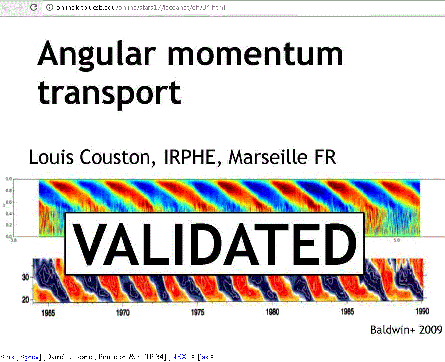
According to Lecoanet and Couston, the large scale fluid dynamics variation is ordered. The small-scale variation (where turbulence is stronger) therefore does not impact natural climate variations. They validated this model against QBO data:
So are you going to retract your statements regarding the impossibility of modeling large-scale fluid dynamics?
”
Back-of-enveloppe-calculation suggests less than a micrometer, assuming all lava went straight into the ocean. Or much less than 1 promille of annual sea level rise.
”
Did you correct for the boil-off and evaporation that occurs when the hot lava first makes contact with the ocean??
Lava shrinkage?
And since all that lava comes from inside the Earth – wouldn’t its radius be reduced, thus increasing sea-level?
No, of course I didn’t. I took a worst case scenario!
But you forgot to allow for the thermal expansion of the ocean due to all that hot lava 🙂 . And for the change in the Earth’s spin axis caused by that mass moving from the centre of the volcano to one flank. And the extra CO2 from burning vegetation which warms the atmosphere and causes even more steric and ice-melt SLR. And of course the CO2 from the volcano itself. Who knows, if you include everything, you might even get it up to one-and-a-half microns!
”
No, of course I didn’t. I took a worst case scenario!
”
Alarmist.
Release your data and code now! – or I’ll FOIA you all the way to the US House Committee on Science, Space & Technology.
RE: the Kilauea lava flow
There might be a related germ of an idea here, but not related to Kilauea —
Coral proxy measurements of ENSO show a ~2x strengthening after 1880-1900 according to the seminal UEP paper by McGregor et al 2010. That’s a mini-hockey-stick shape in the variance
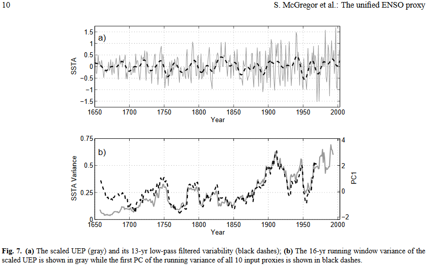
Consider that the Indonesian throughflow is sensitive to tides (see Sprintall et al, 2003). And that the Bali coral record shows significant tidal signals (see Charles et al, 2003).
Could this be Krakatoa-related as the lava perturbed the Sundra strait flow? I agree that the Kilauea event is inconsequential, but with Krakatoa essentially doubling the size of the island in the middle of a critical throughflow strait, that event may have had a climate impact
Probably not. Based, admittedly, on Wiki.
Most of the flow is further east, Only the flow east of Java gets a mention and it’s the smallest of the three final components. So anything west of Java is presumably smaller still. (Krakatoa was only East Of Java in the movie – in the real world it’s west of Java.)
OK Dave, but there is this from “Oceanography Surrounding Krakatau Volcano in the Sunda Strait, Indonesia”, Oceanography, 2016, 29(2):264–272, doi:10.5670/oceanog.2016.31.
Volcanos are trending apparently. Wonderin Willis dashed off another blog post filled with questionable graphs, this time asserting that major volcanic activity does not impact global temperature. From the Oceanography article on Krakatau above
Tomas over at Curry’s is trying to marginalize Nick Stokes’ scientific credentials.
I think the main problem is that those guys don’t seem to understand that chaos theory is an abstract mathematical notion that is not in fact “recognized as a specific field of physics” as Tomas claims.
But it’s seasonal Paul, so reverses with the Monsoon winds. More into the Indian Ocean than out over a year, but look at the numbers. Net annual, a low single figure percentage of the total from the Pacific to the Indian Ocean. I’m all for getting the details right, and I’m sure it’s very important to local navigators, but in the global scheme of things, less than the uncertainty range (or is that year-on-year variation?) in the biggies.
Dave,
Well that’s really a small potatoes thing, as I am able to model the ENSO proxy over a span of more than 365 years via the lunisolar forcing. This is trained on 135 years of instrument data and cross-validated on 230 years of proxy data. So the only minor discrepancy is why the variance changes in the 1880 to 1900 time frame. It could also be a systemic error in how proxies are analyzed, or degradation in the data with age.
Curry’s maddening false equivalency is that she continues to promote horrible guest posts such as from these Hughes&Milanovich characters, who claim that variability is impossible to characterize due to chaos, while she continues to market her own commercial forecasting company that ostensibly claims to be able to predict climate.
Pingback: 2018: A year in review | …and Then There's Physics
An interesting post, and I think what you are highlighting here is a fundamental issue regarding definitions. What is weather and what is climate? This appears to be a distinction that I don’t think many people fully appreciate. But I think you may have identified the key point.
Climate is the steady state solution that depends only on the boundary conditions.
Weather is the time-dependent component that depends on the initial conditions.
If we stick to these definitions then I think the confusion is removed. It also means that chaotic behaviour should be restricted to the weather, not the climate. Ergo, anything that is shown to be chaotic must be weather, not climate.
Except, the next problem is, how do you identify the steady state if the weather component never fully averages to zero, or only does so over an infinite time? This, I think, is the big error climate scientists make. They assume the weather is short-term. It isn’t. Sure, it’s magnitude decreases with time, but it never goes away completely. In which case, how do you know that what you are measuring is climate change and not just long-term weather? Maybe by asking: is what you are observing chaotic?
Possibly… but in addition, well, then there’s physics.
Note to the regulars:
Slarty Bartfast has been displaying his statistical chops recently on this thread over at Skeptical Science, where he seems to feel that he understands weather and climate and time series better than anyone else.
https://skepticalscience.com/2020-SkS-Weekly-News-Roundup_25.html
You may wish to review his demonstrated acumen there before you engage too fully.