I haven’t done a Watt about post for quite some time, so thought I would repeat it just this once. Roger Pielke Sr has guest post on Watts Up With That claiming to present seven very inconvenient questions that Gavin Schmidt is too afraid to answer (yes, I’m going to link to WUWT, deal with it 🙂 ). I’ll ignore the whole rather bizarre “you’re the head of a publicly funded organisation, therefore you need to respond to these questions” framing, and simply address one of Roger’s questions.
Roger refers to a Climate Etc. post, where he discusses an alternative metric to assess global warming. Basically, he just does a simple energy balance calculation which he casts as
Global annual average radiative imbalance [GAARI] = Global annual average radiative forcing [GAARF] + Global annual average radiative feedbacks [GAARFB] (2)
He uses Levitus et al. (2012) to infer a GAARI, since 1955, of 0.39Wm-2 ± 0.031 Wm-2, which is for the oceans only, so it’s increased by 10% to give 0.43Wm-2 ± 0.031 Wm-2. The radiative forcing (GAARF), since 1750, is 2.29Wm-2 (1.13 to 3.33 Wm-2). Since 1950, this becomes 1.72Wm-2. The radiative feedbacks he essentially takes from Soden et al. (2008) and considers the Planck response, water vapour, clouds, and albedo. Together, they sum to -1.21Wm-2K-1. The change in temperature since 1955 is about 0.6K, which gives a net feedback response of -1.21Wm-2K-1 x 0.6K = -0.73Wm-2.
Therefore we have a GAARF of 1.72Wm-2 and a GAARFB of -0.73Wm-2. If we sum these we get 1.72 – 0.73 = 0.99Wm-2, which Roger points out is about twice as large as the value estimated from Levitus et al. (2012). This was one of the things that Roger highlights and asks for Gavin’s best estimates for these terms.
So, why is there an apparent discrepancy between the system heat uptake rate estimated using an energy balance approach, and that estimated from ocean heat content measurements? Well, Roger appears to have made a number of mistakes in his calculation. Firstly, he did not correct for the fact that the oceans are only 70% of the surface. Secondly, it shouldn’t be the global average radiative imbalance, it should be the change in radiative imbalance over the time interval considered (i.e., the difference between what it is at the end of the time interval, and at the beginning). In the most recent decade, Levitus et al. (2012) suggest a radiative imbalance of 0.7Wm-2 (full surface plus increased by 10%). During the earliest decade (1950s) it was probably about 0.2Wm-2. So, the change is around 0.5Wm-2. Roger also forgot to include lapse rate feedback, which – according to Soden et al. (2008) – is probably around -0.75Wm-2K-1. So the feedback is actually -1.96Wm-2K-1, giving a net feedback response of -1.96 x 0.6 = -1.176Wm-2. Combining that with the change in external forcing gives 1.72 – 1.176 = 0.544Wm-2, pretty much the same as that estimated from Levitus et al. (2012). Of course, I’ve just eyeballed some of the numbers, and there are uncertainties to consider, but it certainly seems as though one can come close to reconciling the model-based estimates, and the observations.
So, I think that clears up one of Roger’s questions. The reason for the discrepancy is – I would suggest – simply because Roger’s calculation isn’t correct, not because there really is some kind of major discrepancy between model estimates and observations. Apologies, of course, to Gavin for butting in 🙂
Edit and acknowledgement: I’ve just realised – and Chris Colose has confirmed – that the temperature feedback includes the lapse rate, so Roger’s feeback estimate is about right. However, I still maintain the the correct radiative imbalance is the difference between what it is at the end of the time interval and at the beginning, not the average over the time interval. Hence, the discrepancy is not quite as great as Roger’s calculation suggests.

Funnily enough, I actually had worked on the answer to that one:
A: The post you refer to has a number of very odd statements. First, you seem to think that global mean surface temperature is defined from an energy balance model (Eq. 1). That is backwards. Surface temperature is well-defined field, as is its global mean. The simple energy balance equation you use rather defines a (model-specific) lambda, not delta(T), and your description of its use is highly non-standard. A different specification of the model, for instance, including an ocean box would define a different lambda.
Isaac Held has discussed the difference that the simple model makes in a few of his posts, for instance: http://www.gfdl.noaa.gov/blog/isaac-held/2011/03/11/3-transient-vs-equilibrium-climate-responses/
In any case, the formulation you adopted is one in which surface temperatures are assumed to be in perfect equilibrium with the energy uptake, but that will only be true for fast responses that don’t penetrate beyond the ocean mixed layer. Thus the appropriate sensitivity is not the equilibrium value, but something closer to the Transient Climate Response (which is of course smaller).
There is a rich literature using this equation to estimate TCR (see Otto et al, 2013 for instance). But there are a number of issues that have been raised that undermine its utility. One issue is the assumed constancy of lambda over long time periods. Non-constancy in time is actually very common in GCMs and relates mainly to the difference in response times in the two hemispheres. Deeper ocean mixed layers at reduced ice-albedo land feedbacks in the South slow responses there, and with smaller responses, feedbacks are of course muted eg see Armour et al. (2013). Additionally, there is evidence that different forcings give rise to different lambda’s (e.g. Hansen et al, 2005; Shindell 2014). Our group has been working specifically on exploring this issue in the context of the single forcing CMIP5 runs – stay tuned!
So, to answer your question, I have no problem with the IPCC AR5 assessment of the radiative forcing, though the forcing efficacies should be included if they are to be used in your equation. (NB. You are confused in your statements about the temperature compensation: that does not affect the radiative *forcing* calculation since it is part of the response).
The latest ocean heat content changes from NOAA NODC are reasonable, though likely underestimated slightly due to the sampling issue below 700m depth. You can use any globally complete temperature estimate (GISTEMP, or the enhanced HadCRUT4 data from Cowtan and Way, 2013), and you get a lambda in line with IPCC estimates of TCR (i.e. values equivalent to around 1 to 2ºC).
Gavin,
Thanks, and that’s a nice summary of the whole energy balance approach.
I have some questions for RPjr.
In your testimony before the Senate Environment and Public Works Committee on July 18, 2013 you stated that you performed unpublished study runs that forced a climate model output with increasing Hurricane damage and loss activities that were congruent with high impact scenarios.
You went on to state that even with this forced model result, the statistical significance of the climate driven impacts could not be conclusively determined for “many decades to centuries”.
Question1: How many additional U.S. Atlantic category 3 or greater hurricane landfalls occurred in your model simulations?
Question2: What was the probability of northern migrations of major hurricane landfall events over the course of the model run?
Question3: Assigning a geographically-weighted damage loss estimate per landfall activity, with northern storms generating higher loss values, what was the total cumulative cost estimate of these landfall events before a statistically significant causation could be proven?
Question4: Assigning a likely human mortality per event value to each hurricane landfall in the model, how many Americans would lose their lives before a statistically significant causation could be proven?
[Chill. -W]
Oh no.
Seepage
http://www.theguardian.com/environment/2014/oct/09/why-is-antarctic-sea-ice-at-record-levels-despite-global-warming
What, you agree with Stephan Lewandowsky? 🙂
Roger Pielke Sr.
I found his presumption that Gavin somehow owes him answers to be kinda odd.
It’s even more odd when he poses a question and gets the basis of it wrong.
My mistake I meant
See page
Steven,
Well, yes, I think you pointed something like that out – with regards to the GWPF review – on Climate Etc. recently too. Scientists shouldn’t really be insisting that other scientists do their homework for them.
Maybe I should remind people that this refers to questions posed by Roger Pielke Sr, not Roger Pielke Jr.
I am pleased that one of my questions is being addressed including by Gavin. Needless to say, I will have a more detailed response. I am on travel until Friday and will have a post on this then.
As just two comments here, the oceans uptake more heat than represented by their areal coverage. We did include the same percent adjustment that Jim Hansen has done on this in the past. Second, you are in error in terms of what the global radiative imbalance is. If we accurately sample the Joules in the ocean in say 1950 and subtract the Joules in the ocean in 2015, we can obtain an accurate estimate of the average global average radiative imbalance over this time period. Again, this is the same approach Jim Hansen did as we cited in our post on Climate Etc.
The surface temperature as the primary metric to diagnose global warming is the standard approach used by most in the climate community, but it is not the basic physics approach. With the energy approach we present, we do not need that metric. The heat approach includes mass which the surface temperature as a 2D field does not have. Moreover, we avoid any need to assess a lambda.
More on the issues Gavin and you raised when I have better computer access.
Just one final comment here. If the radiative imbalance is 0.544 Watts meter squared as you calculate, that is still smaller than what Jim Hansen estimated from the GISS model runs for the late 1990s. I do not see either of you discussing that discrepancy.
Regards
Roger Sr
As Jr.’s thing is to send books (or demand you read everything he ever wrote) Sr.’s is to demand answers. A rather amusing example of the Pielke Sr. Gallop was at Real Climate not so long ago and ATTP was involved.
He is also rather fond of playing Humpty Dumpty and proclaiming that words mean exactly what he says they do and not what every other bunny things.
Strange.
Strange to assume that you can give an adult homework.
Strange to expect answers for such a wide range of topics. I know that mitigation sceptics think they have found errors in the science for many specialisations. Scientists normally are more modest and typically master one specialisation.
Strange to put your questions on WUWT. By doing so you signal that you do not think they are valid, otherwise you would publish them in the scientific literature and not on a blog of political extremists known to continually misinform their readers.
Roger,
Thanks for the comment. You say,
This isn’t quite right. Indeed, if we subtract the Joules in the ocean in 2015 from the in 1950, we can determine the average radiative imbalance over the time period. However, from an energy balance perspective, this is not the correct quantity. What we want is the difference between the uptake rate in 2015, and that in 1950. Of course, we can’t determine it instantaneously, so typically (as is done in Otto et al., Lewis & Curry, for example) it is determined as the average rate for the most recent decade considered, and for the base period considered. The change in system uptake rate is then the difference between these two quantities.
This should be fairly obvious. Consider a scenario in which the system starts in equilibrium (i.e., no radiative imabalance) and in which an positive external forcing is then imposed. The system then moves out of equilibrium, and the radiative imbalance will be positive and – at any time – will be the sum of the change in external forcing, the Planck response, and the non-Planck feedback response. Therefore, at any time, the energy balance equation that describes the system is
where is the difference between the radiative imbalance at time
  and time
  . It is not the average rate at which energy is accumulating, it is the difference between the initial accumulation rate, and the accumulation rate at time
  .
.
As the system returns to equilibrium, the radiative imbalance will return to zero. Once it has returned to equilibrium the sum of the change in forcing, the Planck response, and the non-Planck feedback response is, again, zero (i.e., ). The average radiative imbalance is, however, still non-zero since there is a net change in energy (i.e.,
  ). Therefore, once the system has returned to equilibrium, the average radiative imbalance is still non-zero, yet the instantaneous radiative imbalance is zero.
Pass the popcorn.
Thank you for your response. However, you make the issue unnecessarily too complicated. We do not need to express as a temperature response with its lag to heating and cooling. Warming is an accumulation of Joules; cooling is a loss of Joules. We only used surface temperature since we did not have accurate measurements of ocean heat content changes; we do now.
Let’s agree to incorporate and focus on this metric; at the very least elevate it in its importance as a global warming metric ( it should be the primary one, of course).
To further illustrate why the change in heat content provides the robust metric of global warming, consider a pot of water that is heated by a burner. Regardless of whether it is being heated at the start (or just turned on then), if we measured the change in Joules at two time slices, we have the measure of the heat imbalance averaged over that time period.
If we then turn the burner off, the heating stops. There is no lag. There is no “transient response”. No “unrealized heating”, etc. The water starts to cool and we can measure the decrease of Joules, and for any two time slices, diagnose the heat imbalance (cooling).
Roger Sr
P.S. Please refer to Jim Hansen’s analysis of the radiative imbalance that I included in my post on Climate Etc, and see if you can reconcile with your analysis.
Roger,
Yes, I agree that the change in energy over some time interval is a robust metric of global warming. That, however, does not change that at any instant in time, the equation that describes the energy balance of the system is
where is the difference between the energy uptake rate at
  and
and  , not the average energy uptake rate between
  and
and  .
.
So, your question seemed to relate to your estimate in which you computed an energy uptake rate that was quite a bit greater than that observed. Do you at least accept that that that discrepancy was large because the lapse rate feedback was ignored and because the radiative imbalance you computed may have been too small?
You may need to give me a better idea of where to find it, as I’m struggling to do so.
He asked on Watts? Sewage and seepage combined. It can’t be serious, by definition.
The real world was more intriguing today.
http://climatesciencedefensefund.org/new-legal-attacks-on-climate-science-community/
The radiative imbalance we reported remains as we listed (with its uncertainties). On the lapse rate feedback, we had assumed it was included in one of the feedbacks presented in our Climate Etc post. I will check more when I can access those papers (on Friday). If we left off a negative feedback, it would bring the model results in closer agreement.
Now your turn – how do you reconcile Jim Hansen’s estimate of the radiative imbalance even using your analysis,
As to an instantaneous measure of global warming, your equation above is informative in terms of how such warming occurs (a process presentation). However, for accurate measurements of long term global warming (multi decadal) we should take advantage of the oceans as a low pass filter. It does the spatial and temporal integration for us. Why work with differential quantities when we have integral measures?
Global Warming (over multi-decadal time period) ~= Accumulation of Joules in the ocean.
The Real Climate post in 2014 by Stefan R. misrepresented the robustness of that metric.
“To further illustrate why the change in heat content provides the robust metric of global warming, consider a pot of water that is heated by a burner. Regardless of whether it is being heated at the start (or just turned on then), if we measured the change in Joules at two time slices, we have the measure of the heat imbalance averaged over that time period.
If we then turn the burner off, the heating stops. There is no lag. There is no “transient response”. No “unrealized heating”, etc. The water starts to cool and we can measure the decrease of Joules, and for any two time slices, diagnose the heat imbalance (cooling).”
There should certainly be a delay (depending on the “pot”) in the water being heated once the burner is ignited. Why not a lag between the burner being turned off and the cooling of the water? Does it not depend on the physical properties of the “pot?”
For Jim Hansen’s text, please go to our Climate Etc post that is given as a url on my WUWT post of yesterday. The link to Jim’s statements are there. You can also find on my research website in my publications. Do a search for his name.
Sorry I cannot send directly, but it is not as easy to do cut and paste on an iPad as on a laptop. If you cannot find, I will send on Friday as a comment here.
Roger,
Well, you’ll need to give me some link. To be clear, my numbers come from your own source, Levitus et al. (2012). For the period 2000 – 2010, the change in energy is around 1023J. Divide that by the surface are of the earth and by 10 years in seconds, gives 0.62Wm-2. Divide that again by 0.9 under the assumption that only 90% goes into the oceans (which is what you also assumed). During the period 1955-1965, the energy change seemed to be only a few times 1022J, so the average radiative imbalance over that period was a few times smaller than during the period 2000-2010. Hence the difference is around 0.5Wm-2. You used, 0.43Wm-2, so it’s not all that different.
Sure, but that’s not how the energy balance approach works. I’m not disputing that looking at the change in energy in the oceans over a long time interval is a good way to quantify global warming, I’m simply pointing out that if you want to use an energy balance approach, you need to use changes in these quantities, not averages in these quantities.
Okay, I’ll have a look tomorrow, it’s getting rather late here.
Putting aside how these things are calculated, Roger has advocated for years that we use ocean heat storage/changes as a useful metric and indicator of climate change, ‘cuz physics.
To my knowledge, no one has ever said that this is not a useful metric. But he seems to want to replace everything else, a step that doesn’t follow from its utility…it’s just not a complete metric- Stefan actually laid out good reasons for this in his 2014 post. We live at the surface, and much of what we care about and atmospheric responses (e.g., water vapor) care about surface temperature change.
Utilizing the last 4 years of ARGO ocean heat content 0-2000m results the average energy imbalance is between 0.9 and 1.1 W/m^2 depending on attribution of ocean heat vs other system heat response.
I have read Gavin’s response and and remain unclear what he is responding to. We are not using our approach to estimate a global average surface temperature anomaly or any transient or equillibrium response. With the approach we are recommending we avoid any need for computing a surface 2d globally averaged temperature field. Gavin is not discussing the energy budget analysis approach that we did.
Global warming is an accumulation of Joules primarily in the oceans. Does Gavin agree or disagree with this? If we agree, let’s quantify the different components that result in this accumulation of these Joules. That is the basis for the one question being discussed in this post and in our post on Climate Etc with John Christy and Dick McNider.
I also look forward to posts on this weblog on our other questions.
I wonder if Roger knows that real scientists don’t go through the ruminations and brain farts of old blogger posts.
Perhaps he’s referring to Hansen’s 2005 paper;
http://pubs.giss.nasa.gov/abs/ha01110v.html
Roger A. Pielke Sr: Provide actual citations. Not random links du jour.
Chris. I agree we have need to assess surface temperature trends and anomalies. Indeed I have published quite a bit on that subject. I was State Climatologist of Colorado so I am quite familiar with its value.
But as the metric to diagnose global warming, the global average surface temperature anomaly is a very poor substitute when we can use the ocean heat content changes. As to Stefan R. Real Climate post on this metric, he failed to properly present the robustness of this metric. Ask Josh Willis if it is a good metric, for example. Even Gavin seems to agree on its value.
Roger,
Hmmm, okay, I’ve been looking through the Soden papers again and – I may never hear the end of this – but it is possible that the lapse rate feedback is included in the temperature figure. That would mean that your feedback estimate is broadly correct. Certainly, the table 1 here would suggest that Planck plus lapse rate is about -4.2Wm-2. I still think that your estimate for the radiative imbalance is too low as it shouldn’t be the average, it should be the change over the time interval.
Roger,
What Gavin’s point is is that those feedbacks you’re using are over an entire warming interval (i.e, a doubling, or quadrupoling of CO2), whereas your estimate only consider a period over which CO2 has increased by 40%, rather than doubled or quadrupoled. GCMs typically show that these are not constant across the whole doubling or quadrupoling period, and hence using these values to estimate energy balance for a period over which CO2 has not yet doubled can produce a mismatch.
Corey. There is no lag in changes in Joules in the water (and the pot) when the input of Joules stops.
Corey. When the input of Joules from the burner ends, no more Joules can accumulate in the water or pot.
> Therefore we have a GAARF of 1.72Wm-2 and a GAARFB of -0.73Wm-2.
What about the GMAFB?
And than there’s Physics – Then we need the feedbacks up to now. Hard to believe this has not been reported. We used what was available to estimate them. What is your estimate for them them? Seems this is where Gavin can tell us what they are from the GISS model.
ATTB-
The Planck feedback is always about -3.3 W/m2K or so, so the “temperature” kernels are incorporating lapse rate adjustments (i.e., departures from vertical uniform warming) into that.
Yes, I’ve just worked that out myself. I should have noticed that -4.2Wm-2 was higher than I would have expected.
And than there’s Physics. – if you have found a mistake and than acknowledge, my respect for you really goes up. That is a benefit of these Q&A and why I sought to engage Gavin in a discussion. Everyone learns something.
Thanks. I’m going to call this quits for the night, as it really is getting late here.
Also, the whole idea behind radiative kernels is that one should be able to use one pre-computed set of quantities that look like a ∂R/∂x (where R is your TOA radiation and x the feedback of interest) for basically any model that isn’t *too* different…the kernels would likely be sufficiently different in CMIP5-type models vs. an idealized aquaplanet, for example, but since these have been calculated (e.g., Karen Shell or Brian Soden have them available), then Roger could go download GISS model output and determine the feedbacks himself given the actual changes exhibited in those runs.
Roger A. Pileke Sr.:
And than there’s Physics. – if you have found a mistake and than acknowledge, my respect for you really goes up. That is a benefit of these Q&A and why I sought to engage Gavin in a discussion. Everyone learns something.
If you really wanted to engage Gavin Schmidt in a scientific conversation, you would have communicated with him directly rather than by posting your questions on a blog site.
[No suspicious mind reading, please. -W]
All,
Please beware Kurt Vonnegut Jr.’s rule:
http://www.avclub.com/article/15-things-kurt-vonnegut-said-better-than-anyone-el-1858
While this does not preclude physical plays, please try to make sure you can still look your ClimateBall opponent in the eyes at the end of the exchange and shake hands.
ATTP. The accumulation of heat depends on the amount of Joules added over time. The average provides that measure. It is just a use of the mean value of integration (from integral calculus).
John Hartz. See my posting of e-mails between Gavin and I that are posted in the comments section at WUWT. That will answer your question.
Roger A. Pielke Sr: The fact that you and Gavin Schmidt are communicating with each other on a comment thread on WUWT does not tell me why you chose to pose your questions to him in the form of a blog post.
BTW, I assiduously avoid the WUWT website and will not go there to read either your blog post or its comment thread.
Willard: I will bite my tongue as best I can..
Roger, how certain is change in OHC?
When I examine charts of ocean temperature at depth,
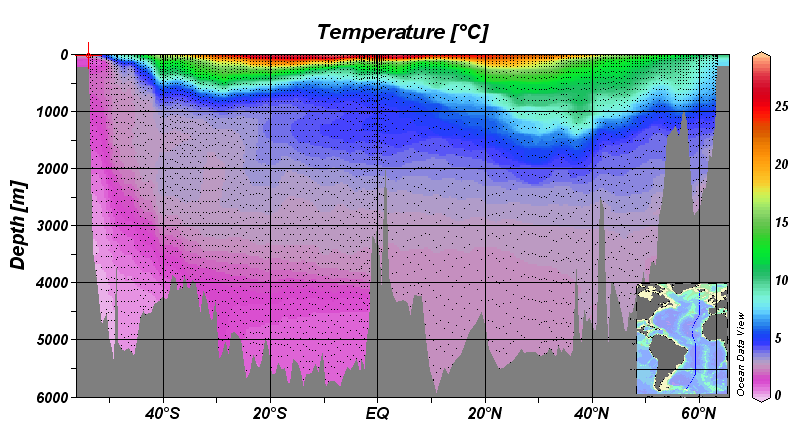
it’s clear:
1. That the average ocean temperature is much lower than the average air temperature because
2. The cold polar regions are unstable and so the oceans differentially store colder waters and
3. The Tropics are the most stable – warming inhibits mixing spatially anyway. It would seem to me
4. Processes involving cold bottom water formation are more important in the long run.
Yes, turbulent exchange does occur.
But what of the question – if turbulent diffusion will mix additional heat downward, why, over the millenia since the last glacial maximum, has average ocean temperature at depth, not approached equilibrium with the much warmer atmosphere already?
RPSr:
“See my posting of e-mails between Gavin and I that are posted in the comments section at WUWT.”
Did you have Gavin’s permission to post his e-mails to WUWT?
The short answer…
Roger forgot to divide by 2
The long answer…
Roger assumes 1950 is in equilibrium, so the additional forcings are relative to 1950 (making 0.57W/m^2 the baseline for anthro forcings, and 2.29W/m^2 the ending forcing in 2011).
The change in total ocean heat content is an integration of the radiative imbalance since 1950 (as Roger says in his May 20, 2015 at 11:16 pm reply)
In other words, total joules accumulated = joules added in 1951 + joules from 1952… 1953… up to the last year in question (2011)
The radiative imbalance for the last year (2011) = +1.72W/m^2 from the 2011 net anthro forcing – 0.73W/m^ for 2010 net feedback = +0.99W/m^2
The radiative imbalance for the first year… 1951… is anthro forcing for 1951 (a small positive number relative to the 1950 baseline) – 1.21W/m^2 * (delta temp). The delta temp for 1951 is also a small number, so the net imbalance in 1951 is very small – close to zero, not 0.99W/m^2.
If we assume both temps and anthro forcing have increased linearly since 1950, we can approximate the total integration by averaging the 1951 and the 2011 imbalances.
Therefore…
GAARF = (1.72 + ~zero)/2
GARRFB = (0.73 + ~zero)/2
average net imbalance for 1950 to 2010 = 1.72/2 – 0.73/2 = 0.495W/m^2
vs 0.43W/m^2 from OHC calculation.
Close enough for government work. If you go back and calculate the actual net imbalance for each year, add them up, divide by number of years to find the average, maybe it is closer to 0.43W/m^2, since the temps and forcings increased slower than linearly at the beginning.
…
Let me shamefully repost the comment I had addressed to Roger Sr. on Climate Etc. last year:
Roger Sr.,
I went through your calculation and I have two issues.
For purpose of calculating GAARFB you are using the 2.99W/°Km2 from Wielicki et al. 2013. I haven’t read that paper but it’s easy to calculate that such a value for the climate feedbacks yields a sensitivity of 3.05°K per CO2 doubling equivalent (assuming 3.7W/m2 forcing from a CO2 doubling). Hence your result purports to show that the radiative imbalance (from Levitus et al.) only is half what one would expect if climate sensitivity were 3.05°K. Though this is the middle of the range for IPCC estimates of ECS, I think a 2°C TCR is a better point of comparison for the climate response to the forcing change since 1955. I also think the IPCC projections for 2100 are based on models that have a TCR response closer to 2°C/CO2 doubling in that time frame than to the full equilibrium response.
If we calculate the expected imbalance with a climate feedback value of 2.35W/Km2, which corresponds to a TCS of 2°C/CO2 doubling, then, for a 0.6°C temperature rise, we get a resulting imbalance of just 0.61W/m2.
My second issue concerns your tacit assumption that the current imbalance that you calculate ought to reflect the average imbalance over the 1955-2010 period. This is the 0.39W/m2 from Levitus et al. (2012). But your GAARI = GAARF + GARFB equation only is valid for the value of those parameters at any point in time (or as yearly averages over specific years). It would also hold exactly over the whole period, since it is linear, if you would average *all* the terms. But what you do is average only GAARI while using the end values for the right hand side of the equation. It is however to be expected that — (assuming as you do, for simplicity, that there is no significant imbalance in 1955) — as the forcing increases, the imbalance will not immediately jump to its average value over the whole period that ends in 2010. Rather, it will grow progressively and can be expected to be higher at the end of the period than its average value. Indeed the estimates of the increase in ocean heat content over recent periods 1990 until 2008 might have ranged from 0.46 to 0.73W/m2 +- 0.16W/m2 (Nuccitelli et al. 2012).
So, the observed recent imbalance seems to be fully consistent — indeed in the middle of the uncertainty range — with what one would expect if the TCS were 2.0°K/CO2 doubling.
“Let me shamefully repost…”
Shamelessly, that is…
Turbulent Eddy. The ocean research community has placed uncertainty estimates on their heat change analyses. The data, particularly in the upper 700m, is quite good particularly since 2003.
Wehappyfew. Nope. No divide by 2 required.
TE,
The oceans are stratified for a reason, it’s called the AMOC. We also happen to live in an ice age and are currently at an interglacial cycle which has followed ~100K years glacial cycle. We also still have two rather large pieces of ice located near the upwelling and downwelling zones, you may have heard of these largish pieces of ice, the’re in the polar regions, it’s usually below freezing up/down there, but stuff melts the waters warm the water sinks yadda yadda yadda, or so I’ve been told.
Outside of the upwelling and downwelling zones you need a vertical velocity gradient greater than the buoyant restoring force to mix two horizontal layers (cold abysmal ocean and warm surface ocean), some people call this a densiometric Froude number or gradient Richardson number (basically a dimensionless parameter of the buoyant restoring force to inertia overturning force, or the shear gradient to density gradient yadda yadda yadda).
The key takeaway is stratification.
I’m quite sure I have not answered your question.
I seriously doubt that I, or anyone else for that matter, could answer your question to your own satisfaction, given your own track record here. D’oh!
But maybe, Roger will be kind enough to provide a few dozen references where he ‘just’ happens to be one of the authors, Roger is very good that way, he really likes referencing himself, or so I’ve been told.
Roger,
I realize you are a very busy and very famous internet scientist, but a more reasoned and mathematically complete counter-argument than “nope” would be greatly appreciated.
Let me try another re-wording of the problem…
you said this on JC’s blog in 2014…
> “If we assume that all of the radiative forcing up to 1950 has already resulted in feedbacks
> which remove this net positive forcing, the remaining mean estimate for the current
> GAARF is 1.72 W m-2.”
….
You’ve defined the net radiative imbalance for 1950 to be zero, as it is assumed to be in equilibrium – radiative forcings and radiative feedbacks are balanced, and we are only concerned with the additional 1.72W/m^2 forcing that has accrued since 1950.
Therefore the total contribution to OHC for the year 1950 is ZERO joules, correct? If my reasoning here is wrong, then my argument is wrong, and yours is correct, so you must verify this question first…
Equilibrium in 1950 means no net joules entering the ocean… do you agree?
The radiative forcings increase from zero in 1950 to 1.72W/m^2 in 2011.
The radiative feedbacks “increase” from zero in 1950 to -0.73W/m^2 in 2011.
So both terms are increasing from zero in 1950 to their final value in 2011. Each year in between 1950 and 2011 has some intermediate value.
…
For example, in 1980, the additional radiative forcing was 1.25W/m^2 – 0.57W/m^2 = 0.68W/m^2
(1980’s value minus 1950’s value)
The additional radiative feedback in 1980 would be 1.21W/m^2/degK * (delta temp from 1950 to 1980) = 1.21 * 0.3 = 0.363W/m^2
The radiative imbalance for 1980 would therefore be 0.68 – 0.363 = +0.317W/m^2
Do you agree?
…
This is a long-winded way of saying that the total quantity of joules deposited in the ocean since 1950 is the sum of the joules deposited during each intervening year. The AVERAGE radiative imbalance is found by summing the imbalance for each year and dividing by the number of years.
We know the exact values for 3 of these 61 years…
1950 = zero joules entering the ocean = 0.0W/m^2
1980 = 0.317W/m^2
2011 = 0.99W/m^2
Averaging just those 3 years, the AVERAGE radiative imbalance = 0.436W/m^2
All the years in between 1950 and 1980 will be greater than zero, less than 0.317W/m^2. All of the years between 1980 and 2011 will be greater than 0.317 and less than 0.99W/m^2… the average for all 61 years will be close to 0.43W/m^2.
According to your calculation, the AVERAGE value for a series that increases continuously from zero in 1950, to 0.317W/m^2 in 1980, to 0.99W/m^2 in 2011 = 0.99W/m^2.
I think that is mathematically unsupportable.
Please show more mathematical reasoning than “nope” to show how you calculate that average.
Thanks.
…
Roger,
Yes, you’re saying something true, but that isn’t relevant to your calculation. Your calculation in the Climate Etc. post is an energy balance calculation. In such a calculation, you’re balancing the change in forcing, with the feedback response, and the difference between these is the change in radiative imbalance, not the average of the radiative imbalance.
Consider what it says in the Supplementary Information in Otto et al. (2013), for example,
So, it’s the difference, not the average over the full time interval.
They even say
There are a couple of other things to bear in mind. Since the heat uptake rates are potentially decadal averages, you should really use decadel averages for the temperature and change in forcing. Also, the surface doesn’t equilibrate instantly with the upper ocean, so a small lag (a few years) between the change in forcing and change in temperature is reasonable. Also, as Gavin points out, the feedbacks aren’t typically constant over the entire time interval during with the system returns to equilibrium. Plus, there are of course the uncertainties to also consider.
Roger might ask himself how long his model would take to reach its current equilibrium if the run started with realistic initial conditions, with the sun just starting to fuse hydrogen, and the earth’s bulk temperature set to 4.6 K match the cosmic background .
Forget the ocean thermal mass- it’s the R value of 4,000 kilometers of olivine that matters
TurbEd
Because the downwelling water at high North latitude is very cold already having lost much energy to the atmosphere already by this stage in its journey North. This is the water that forms the deep returning leg of the NH THC (pole -> equator). It provides a continuous supply of cold deep water to the mid- and equatorial latitude oceans.
wehappyfew,
I think even you’re not quite correct. As you say, we can assume that we start in equilibrium, therefore all quanties are initially zero. We then impose some change in radiative forcing (external). That produces a planetary energy imbalance, which warms the surface and produces a feedback response. At any instant in time, the energy balance is then
where is the current planetary energy imbalance (since it started at zero),
  is the change in radiative forcing, and
  is the feedback response.
So, at any instant in time, the rate at which we’re still accruing energy (the radiative imbalance) is the difference between the change in forcing (external) and the net feedback response. Of course, in practice, we would consider some reasonable time interval (decade) over which to average these quantities.
I thought I would post a link to the RealClimate post that discusses the time dependence of the feedbacks. Essentially, if you consider some initial change in forcing, then
So, if you were to divide your initial change in forcing into equal sub-intervals, the warming per change in sub-forcing is smaller initially, than later. So, overall, if you consider that the actual radiative imbalance today is probably around 0.7Wm-2 (or maybe even slightly larger) and that the average feedback response is probably greater than the initial feedback response, the discrepancy is not as large as Roger’s calculation suggests.
I am surprised how somebody with the background of Pielke Sr does not seem to get the importance of the variability in ocean heat uptake and of physical processes like those described in England2014, and I am worried it could be related to dumbing-down sites like WUWT.
Catalin (and ATTP),
Some ancient history. We had this on SKS many years ago re the variability in OHC. Typically of climateball, nothing has changed in the intervening time…
My challenges to Pielke as to the accuracy of OHC:
http://www.skepticalscience.com/news.php?p=2&t=226&&n=357#24092
http://www.skepticalscience.com/news.php?p=3&t=226&&n=357#24242
Pielke appears to confirm he really does claim monthly data is good enough(!):
http://www.skepticalscience.com/news.php?p=4&t=226&&n=357#24328
On further challenge Pielke seems to avoid the question:
http://www.skepticalscience.com/news.php?p=4&t=226&&n=357#24509
My final word:
ATTP. If the discrepancy is not as large as we calculated, use the framework that we provided to show that. I do not know, however, how you conclude the current annual averaged radiative imbalance is 0.7 Wm-2 or slightly larger. After justifying with the ocean heat uptake data, however, use that in your analysis. As to the equation we use, it is an energy conservation statement. It is a basic physics truth. Please use the pot of water example I gave to show how this is incorrect.
On Jim Hansen’s comments, have you been able to find that url on my website?
Roger Sr
aTTP,
I don’t see any conflict between your equation for the instantaneous energy imbalance versus my estimate of the _average_ energy imbalance from 1950 to 2011.
We know the imbalance for three years… 1950, 1980, and 2011.
Roger calculates the imbalance for 2011 and assumes that average applies for all the other years, when we already know that 1980 is 1/3rd as big.
Look again at the chart Roger posted at Judy’s, taken from IPCC – Figure SPM.5 – it shows the “net anthropogenic RF” for 1980 to be 1.25W/m^2, and 2.29W/m^2 for 2011.
for the 1980 imbalance, relative to the assumed 1950 equilibrium:
forcings – feedback = imbalance
(1.25 – 0.57)W/m^2 – 1.21W/m^2/K * deltaTemp = +0.317W/m^2
Roger is ignoring the intermediate value… for 1980… using only the last value… for 2011… and calling that the average radiative forcing for the whole 61 years. And he uses the final temperature to calculate the average feedback response.
This is the underlying mistake… the energy imbalance for each year is what contributes heat to the OHC for that year. That imbalance varies as the forcings and temperature feedbacks vary… from 0.0W/m^2 in 1950… to 0.317W/m^2 in 1980… to 0.99W/m^2 in 2011… but Roger uses only the last year’s value as the average for the entire 61 years.
That’s a basic math error. Pierre-Normand pointed this out on May 6 2014, in the comments to Roger’s article at Judy’s. Roger ignored it. Today his counter-argument is “nope”.
…
Roger,
Well, the current NOAA update suggests that we’ve accrued about 1023J in the last decade or so. Therefore, we can write
If this is 90% of the uptake rate, then the system heat uptake rate is 0.69Wm-2. As Gavin says, though,
So, maybe it could be a bit above this. I wouldn’t want to claim that this is definitively true, but I was just basing it on what seems to be a reasonable statement by Gavin about the measurements below 700m.
Yes, I agree, but I still maintain that in the following equation (which is essentially your formalism)
the term is the change in system heat uptake rate over the time interval considered, not the average rate over that time interval. If you use the average, then if we are warming it will only go to zero as
  , which doesn’t really make energetic sense.
I haven’t yet found Hansen’s statement but I don’t disagree with your claims about how to quantify global warming, I’m simply suggesting that the energy balance formalism requires the change in radiative imbalance, not the average of the radiative imbalance.
Wehappyfew. There is no assumption as to what the radiative imbalance is in 1950. What needs to be done is to measure the heat content in 1950 and the heat content in 2015 and take the difference. These added Joules were added at a rate that changed over time. Using the mean value of integral calculus, we can obtain an average rate that gives us the same answer. We can do this for any time slice. This is quite straightforward.
This rate (energy imbalance) is due to two terms: forcing and feedback. This then is the budget equation.
Roger Sr
Roger,
Well, I would just suggest that your 0.43Wm-2 should really be 0.7Wm-2 minus whatever the uptake rate was at the beginning of your time interval (i.e., the average for 1955-1965 for example). I estimated that to be around 0.2Wm-2, so the difference is 0.5Wm-2, not 0.43Wm-2. Similarly, you should also be averaging the change in forcing over those same two time intervals and also the temperature. Otto, for example, estimate the average change in forcing for the 2000s – relative to 1750 – to be about 1.95Wm-2, so smaller than the 2.29Wm-2 that you used. If I look at their supplementary information (Figure S1), it would seem that a reasonable estimate for the change in temperature (average of 2000s minus average for 1955-1965) would be about 0.45K. So, if I redo your calc, I get
So, a little closer to my estimate of around 0.5Wm-2. Again, there are uncertainties and things to consider.
I should make clear that I’m not disputing a discrepancy (that’s been self-evident since people starting publishing these energy balance calculations and should probably have made me think about the result I first got in this post) simply that it may not be as large as your calculation suggests.
Roger,
Except this is an instantaneous representation of the energy budget, not an average representation of the energy budget.
wehappyfew,
Maybe I misunderstood your point, because I certainly agree with this.
Verytallguy. Physics still have not changed since then. I also do not post comments on SKS any more since it is not interested in courteous discussion of issues. I am finding ATTP refreshing even though we still disagree on a few issues.
Wehappyfew. I am really puzzled how the straightforward conservation equation for heat can be made so complicated. If we measure the heat content in 2015 and in 2014, we can obtain the radiative imbalance for the one year. We can do for one month if the data is good enough (e.g. for an illustration of this see the Ellis et al paper I cited in my BAMS article on this subject where the annual cycle is shown).
We can measure in 1950 and 2015 also.
The radiative imbalance between any two time slices is due to two terms: forcing and feedback. There is an uncertainty, of course, but since 2003 the data is quite robust particularly in the upper 700m.
Roger,
“We can do this for any time slice. This is quite straightforward.”
Then do the same calculation for the time slice from 1950 to 1980.
You can get the OHC from NOAA.
From the SPM.5 chart, the net RF is (1.25 – 0.57)W/m^2
The net feedback is -1.21W/m^2/K * deltaTemp
deltaTemp from 1950 to 1980 is about 0.3degC
I get 0.317W/m^2 for the imbalance calculated using the 1980 RF and feedback values… what do you get?
For the OHC change from 1950 to 1980, it looks like about 10.5 *10^22 Joules from the NOAA data here:
http://data.nodc.noaa.gov/woa/DATA_ANALYSIS/3M_HEAT_CONTENT/DATA/basin/pentad/pent_h22-w0-2000m.dat
(if we assume not much change from 1950 to 1957)
10.5 *10^22 Joules/23 years/ocean area = 0.4W/m^2
…
I agree the rate varies, and now you admit that it does as well. That’s a little progress. The rate was much lower in 1980, as calculated above.
…
Your definitions of GARRI, GAARF, and GAARFB have the units of ” Joules per time period (and can be expressed as Watts per area)” as you stated in your article.
But your _actual calculation_ of GAARF and GAARFB uses the values valid during the time period for 2011, not the average for the entire time period 1950 to 2011.
…
“There is no assumption as to what the radiative imbalance is in 1950.”
This directly contradicts what you wrote in your article…
“If we assume that all of the radiative forcing up to 1950 has already resulted in feedbacks which remove this net positive forcing”
Feedbacks which remove the forcing up to 1950 is exactly the same as saying the forcing and feedbacks were equal in 1950.
If forcings and feedbacks were equal in 1950, as you directly state, then there was zero imbalance. There was an equilibrium…. 0.0W/m^2 added to OHC for that year.
…
Roger,
No, this isn’t quite right. Consider the following. At time , we have a radiative imbalance of
  , and let’s assume that the forcing is measured relative to this time (i.e., the forcings and feedbacks are zero at
  ). If at time
  , the external forcing has increased by
  (i.e., it has increased by
  between
  and
and  ), then the feedback response will be
  , where
  is the change in temperature between
  and
and  .
.
The radiative imbalance, , at
, at  will therefore be
which we can rewrite as
Therefore the change in forcing plus the feedback response represents the change in radiative imbalance, not the average of the radiative imbalance.
ATTP. Go to Other Selected Papers on my research website and search for Hansen. Look for his “Response”
Roger,
You mean, this. Seems fine to me, and seems rather consistent with what I’ve been saying. They say
If “by the end of the decade” they mean around 2010, then if I consider the NOAA data for the period 2000-2010, I get a change of around 1023J, which would be an average for the decade of around (as I showed above) 0.7Wm-2. Less than their 0.85Wm-2, but not hugely discrepant.
ATTP. The use of two time slices only gives us the average heat input over those two time periods. It does not give us the change over this time period. It does not tell us the forcing or feedbacks at the end time slice or at the beginning.
However, it does tell us the average global warming between the two time slices. Agreed?
Now we can do this for 2014 and 2015 (a one year time slice). We can then obtain an evaluation of global warming over that one year time period. Do you agree?
For these time slices, we can estimate the forcings and feedbacks in this time period.
We provided estimates for the forcings and feedbacks for the time slices we used in Climate Etc. Use other values if you feel needed. I agree they need to be refined and urged Gavin to do this for years (which he has still not done).
But realize that the observed radiative imbalance based on the ocean heat uptake is a real world constraint that the forcings and feedbacks must fit into.
Roger Sr
ATTP that is the article. The end of the decade meant 1999.
Roger,
No, I don’t quite agree. The definition of a change in forcing is exactly that, a change in forcing. The feedback response is similarly a change, not an average.
No, I don’t think I do. If you know the change in forcing over some time interval, and you know the feedback response over that time interval, that tells you how the system heat uptake rate has changed. If you wanted to actually know how much energy has accrued you would really need to integrate over that time interval, not simply take a difference. This is essentially – I think – what wehappyfew is pointing out.
Yes, but forcings and feedbacks are driving us back towards energy equilibrium. What is relevant, therefore, is how the radiative imbalance is changing with time, not how the average of the radiative imbalance is changing with time.
Roger,
Okay, then the NOAA data might suggest that the average for the 1990s was a little smaller than the average for the 2000s.
Roger,
I’ll ask you a specific question that might clarify this. Consider the following:
a system starts in equilibrium, with no planetary energy imbalance. We apply a change in radiative forcing. Over sime time interval, t, the system warms, feedbacks operate, and it returns to energy equilibrium. At time t:
1. What is the planetary energy imbalance?
2. What is the average of the change in energy between 0 and t?
Roger,
And as I said on that thread, despite not being able to agree with your conclusions (in that case on the ability of OHC data to give an accurate month- by – month account of the global heat balance) I very much appreciated your engagement in the thread there, and I’d repeat that here.
I think you have enough interrogators here already, however so I’ll not pile on.
Your pithy sense of humour in simultaneously rejecting SKS for being discourteous and posting at WUWT comes through wonderfully – the climate debate could do with being a little more light hearted sometimes!
I’m glad you enjoy the discourse here, please continue.
ATTP. If I have no money at time zero and 100€ at a later time, say 100 hours, I have added 100€ to my budget. I cannot say anything about the rate it was given to me; just that the average is one € per hour. Maybe it was given to me in the last hour. If so the average is not a good representation of what occured.
But if I had data for the each hour, I could.
This is analogous to what we are doing with the ocean heat uptake data.
Also, I look forward to your discussion of Jim Hansen’s statement. It does appear the GISS model, while it did a good job in the 1990s, over predicted the radiative imbalance in recent years. Seems this needs to be recognized and explained.
Roger P.
ATTP. On your example, please give me numbers to use. Specifically, give me the Joules added over time. That is where I will start. Roger Sr
Verytallguy. I do read SKS posts, however. 🙂 WUWT does provide a forum that is widely read; would SKS have posted what I wrote on WUWT? If so, I encourage them to repost and address the questions I have raised. I would even comment then if they permitted an open discussion.
“ATTP. On your example, please give me numbers to use. Specifically, give me the Joules added over time. That is where I will start.”
Why not just write the equations? Numbers can come later.
Pre-ARGO.
Roger,
If the discrepancy is not as large as we calculated, use the framework that we provided to show that.
Surely the best thing to check would be what the actual models produce in direct relation to the observation system you’ve used. See Errata Figure 9.17 http://www.climatechange2013.org/images/report/WG1AR5_Errata_17042015.pdf
The mean 1960-present increase for total ocean is about 24 10^22J, similar to the Levitus 2012 result 0-2000m result.
> Physics still have not changed since then. I also do not post comments on SKS any more since it is not interested in courteous discussion of issues.
In what way is your title at Tony’s courteous to Gavin, may I ask?
In fact, in what way is Tony’s courteous at all?
Roger,
Yes, I agree with this, obviously. However, this doesn’t include the forcings and feedback analogy. They would be equivalent to you starting in a state, where your expenses match your income. Your income then starts rising, and your expenses lag, but grow. Therefore if you know your income and your expenses at any future time, you know the rate at which you are adding money to your account, but not the average rate at which you’ve done so.
That’s the difference. The forcings and feedbacks are more like how your income and expenditure has changed, and hence they – by themselves – do not tell you the average rate at which your account is growing, but the difference between the rate at which it is growing now and the rate at the beginning.
Roger,
Well, I don’t need to for you to answer the question, but let’s assume that at t = 0, it was 0, and at t = t it is E.
As far as this goes, you may need to give me some more context, because I don’t have anything really to say about Hansen’s comment. I agree that there appears to have been an over-prediction in that particular model, but I don’t think it’s quite as great as you suggest. It would be interesting to look at some of the other models, but I’m rather short of time at the moment.
Paul S.,
Thanks. That would seem to be a reasonable response to at least one of Roger’s questions.
ATTP If E is the amount of Joules added, than the rate is average rate is E/t. In your example, this is clearly not an accurate measure at most time periods. If we sample in the last 10% of the time period, the energy input would be smaller, approaching a rate of zero at the end. At the end period, there is more heat in the system but the imbalance has gone to zero.
Than, one needs to reconcile this with the best estimates of the forcings and feedbacks over this time period.
This approach is what we did. In the real world example, where the CO2 and other greenhouse gas concentrations are increasing, E should be increasing in response. We used the IPCC estimates of the total radiative forcings to do this (and these number certainly need to be adjusted to the current 2015 value – this is another item I have asked Gavin about in the past). Give your best estimate of the CO2 and other radiative forcings for 2015. Same for feedback values,
At least we now agree that Jim Hansen’s value is too large for the last decade or more. How large a disagreement you see?
Roger Sr.
Willard – I agree with you. The header was snarky and unnecesasary. I did not write that. My header would be Questions for Gavin Schmidt, Director of GISS.
I respect Gavin, even though I fail to understand why he himself is often not constructive in this interactions. Indeed, he does not seem to understand that by engaging on the questions we have raised he will improve GISS as an honest broker of the diversity of scientific perspectives.
Thank you.
Roger,
Well, yes, so the average over the time interval t, is non-zero, but the radiative imbalance at the beginning and at the end are both zero.
Well, not really. If it starts in energy equilibrium/balance and ends in energy equilibrium/balance, then the change in forcing has to match the feedback response, by definition. Therefore, the change in forcing minus the feedback response is zero, but the average radiative imbalance over the time t is non-zero.
From the NOAA data, I would estimate a radiative imbalance of 0.7Wm-2 against his projected value of 0.85Wm-2.
However, as Paul S indicates, the CMIP5 average is pretty close to the Levitus et al. (2012) measurements.
ATTP – You want the radiative imbalance in 2015 and the 2015 radiative forcings and feedbacks.. I would like that too. Satellites have been used for these, but have very large uncertainties. Using the 2014-2015 ocean heat content change gives us a good estimate of the imbalance.
What is your estimate for the current forcing and feedbacks and how did you estimate them?
Roger Sr
Roger,
I think we may be heading towards a discussion we’ve had before. By definition a forcing is a change over some time interval. Similarly, the feedback will be the response over a time interval (over which the temperature changes by some amount). This seems to be the crux of the issue. In 2015, we can estimate – relative to some earlier time – the change in forcing and, given the change in temperature over that time interval, the feedback response. The difference between these two quantities is the difference between the system heat uptake rate now and what it was at the beginning of the time interval.
In some sense, it doesn’t even make sense to ask what the forcing and feedbacks are in 2015 since they are – by definition – defined as the change over some time interval.
ATTP Jim Hansen’s estimate was for the end of the 1990s. It would be larger now using his approach. Also, realize that any heat that goes into the deeper ocean is not going to be available to affect weather on multi-decadal time scales. It is effectively a sink. It also is not going to be captured by a surface temperature trend.
If you elect to use 0.7 Watts per meter squared as the current imbalance, what is the current radiative forcing and feedback in the same units? What does the GISS and other models produce in terms of their simulated radiative imbalance?
In your example, over the time period, the forcing is equal but opposite in sign to the feedbacks. I agree; but do not see your point as this interpretation of heating is exactly what we did.
Roger Sr.
Roger,
I did that calculation here. I also maintain that forcings and feedbacks are only defined relative to some baseline state. What you seem to be asking for are the abolute energy fluxes, which are not quite the same thing.
My point is simply that the difference between the change in forcing over some time interval and the feedback response is the change in radiative imbalance, not the average of the radiative imbalance.
If we go back to the bank analogy. If you know how much your income has increased by over some time interval, and you also know how much your expenses have increased by, then you can determine the change in the rate at which the money in your account is growing, but you can’t determine how much it has grown by – for that you would need to intergrate the difference between your income and expenditure over time.
I’ll write what I was suggesting in equation form.
[Keep your seeming to you and chill. -W]
Last time I looked it was May 2015. A new OHC record has been set each successive year between 2008 and 2014, and since 2005 the OHC has doubled. This is clearly an inconvenient truth for Pielke Sr. et al.
Moreover, the following misleading statement shows that Pielke Sr is clearly stuck in the past,
“At least we now agree that Jim Hansen’s value is too large for the last decade or more”
That assertion is just begging to be quote mined by someone like David Rose. Further, that assertion may have been true for a past period of time and for one particular model and one particular model integration, but again, it is May 2015 and the data show Pielke’s assertion to be demonstrably false 😉 He is cherry picking again.
Speaking of which, while we have Roger’s attention, will he finally concede that he was wrong to try and have people believe that global sea levels stopped rising circa 2006? Google it and you’ll find his claim, RealClimate has a nice debunking. Unfortunately for Pielke Sr., observations show that since 2006 the average sea level has risen by over 3 cm (or about 40% of the increase between 1993 and present) and findings in a recent paper in Nature Climate Change (by Watson et al.) indicate that sea-level rise has likely accelerated.
[Useless speculation about intention. -W]
Thanks!
Roger asks,
“What does the GISS and other models produce in terms of their simulated radiative imbalance?”
Really? Why doesn’t Roger go [… Unnecessary roughness. -W] download the data (or digitize some graphs like the ones from AR5 provided by Paul S. above) and get back to us with the results?! The data for multiple models are all there for goodness’ sakes.
It is annoying (and reflects poorly on Roger) when he insists on asking others to do the science for him. Really, this sort of analysis is not difficult, yet Roger keeps refraining from actually doing the work.
And so we all continue to do a merry dance and fiddle while Rome burns…
Thanks!
“So, I think that clears up one of Roger’s questions.”
Thank you. It is in the answering of questions that the “show your work” aspect is revealed. I do it regularly even when I know that the question was not asked in good faith.
You exemplify the claim that scientists do and should regularly try to find errors in others’ work; not that they are doing it for high moral reasons but it gets the job done.
I suspect that some of these questions are a gambit to show whether the targeted person can answer them. If you can and he cannot then maybe the wrong person is in the director’s chair. I’ve had a few people claim as their work, mine, and rode that claim to promotion. Whether that’s true here is not for me to say but this “gambit” exposes the possibility.
ATTP: How accurate is the basic assumption that the oceans absorb 90% of the heat? How sensititve are Roger Pielke Sr’s calculations to this assumption? In other words, what is the impact of assuming this percentage to be 89%? 91%?
JH,
A few percent really. It’s typically taken to be 93%, so my estimate would drop from 0.69Wm-2, to 0.67Wm-2. I’d like to think we’re not arguing over a few hundreths of a Wm-2 :-).
Roger,
I vaguely recall ( though I can’t find the link ) Isaac Held contemplating diabatic versus adiabatic contributions to OHC. Do you have an insight into what portion of the assessed OHC change may actually be adibatic?
TE,
What do you mean by “adiabatic” in this context? In fact, I’m not even quite sure what “diabatic” means.
Ocean water is “semi-compressible” and when “semi-compressed” will warm.
But this warming is reversed when such waters are uncompressed (adiabatic) as opposed to heating from the surface or sunlight (diabatic).
Variations of such processes are occurring constantly due to circulation changes.
But to what extent? and over what time scales?
> Speaking of which, while we have Roger’s attention […]
Why not refrain from playing the man, if only to preserve that attention for a change?
If all there is on the table are science moves, the harder will it become to escape from science running its course.
Let’s fill in some real numbers to Roger’s variables.
GAARFB depends only on temperature so it is easy to calculate. We want the change from 1950, since he assumes all forcings and feedbacks before that have equalized.
Average NOAA Land+Sea temps by decade:
1945-1954 = -0.022 Lets use this as the baseline to represent the 1950 equilibrium
1955-1964 = 0.026
1965-1974 = 0.034
1975-1984 = 0.152
1985-1994 = 0.287
1995-2004 = 0.518
2005-2014 = 0.602
Subtracting the 1945-1954 average to get the difference from the 1950 baseline:
1945-1954 = 0
1955-1964 = 0.048
1965-1974 = 0.056
1975-1984 = 0.174
1985-1994 = 0.309
1995-2004 = 0.54
2005-2014 = 0.624
We can calculate GAARFB with the formula: -1.21W/m^2/K * deltaTemp = GAARFB
So GAARFB for each decade:
1945-1954 = -0.00 W/m^2
1955-1964 = -0.06 W/m^2
1965-1974 = -0.07 W/m^2
1975-1984 = -0.21 W/m^2
1985-1994 = -0.37 W/m^2
1995-2004 = -0.65 W/m^2
2005-2014 = -0.76 W/m^2
We also know the GAARF for 1950, 1980 and 2011
1950 = 0.0 W/m^2
1980 = 0.68 W/m^2
2011 = 1.72 W/m^2
Putting it all together, if we assume the GAARF is approximately valid for the decade around it, we can calculate GAARI:
for each decade… GAARF – GAARFB = GAARI
1945-1954 0.00 – 0.00 = 0.00 W/m^2
1955-1964 ? – 0.06 = ? W/m^2
1965-1974 ? – 0.07 = ? W/m^2
1975-1984 0.68 – 0.21 = 0.47 W/m^2
1985-1994 ? – 0.37 = ? W/m^2
1995-2004 ? – 0.65 = ? W/m^2
2005-2014 1.72 – 0.76 = 0.96 W/m^2
We need just 4 numbers to make a fairly accurate approximation of the AVERAGE GAARI from 1950 to 2011.
…
BTW, if you think we have a clear understanding of the processes of OHC storage of surface heat, think again.
Here are a number of AR4 models of OHC from this Roy Spencer post.

This was a model of the past ( 1955 through 1999 ). The models appear to be worthless:
AARGH… formatting…. maybe this will be more readable:
…for each decade… GAARF – GAARFB = GAARI
1945-1954 0.00 – 0.00 = 0.00 W/m^2
1955-1964 ???? – 0.06 = ??? W/m^2
1965-1974 ???? – 0.07 = ??? W/m^2
1975-1984 0.68 – 0.21 = 0.47 W/m^2
1985-1994 ???? – 0.37 = ??? W/m^2
1995-2004 ???? – 0.65 = ??? W/m^2
2005-2014 1.72 – 0.76 = 0.96 W/m^2
Turbulent Eddie,
Temperature is converted to potential temperature before calculating heat content, so zero is related to those processes… in theory. In practice obviously correcting for pressure is a source of uncertainty in the observations.
Roger A Pielke Sr.:
You state:
ATTP Jim Hansen’s estimate was for the end of the 1990s. It would be larger now using his approach. Also, realize that any heat that goes into the deeper ocean is not going to be available to affect weather on multi-decadal time scales. It is effectively a sink. It also is not going to be captured by a surface temperature trend.
How does your statement about deep ocean heat square with the new research findings summarized in the following article?
The world’s oceans are playing a game of hot potato with the excess heat trapped by greenhouse gas emissions.
Scientists have zeroed in on the tropical Pacific as a major player in taking up that heat. But while it might have held that heat for a bit, new research shows that the Pacific has passed the potato to the Indian Ocean, which has seen an unprecedented rise in heat content over the past decade.
The new work builds on a series of papers that have tracked the causes for what’s been dubbed the global warming slowdown, a period over the past 15 years that has seen surface temperatures rise slower than they did the previous decade. Shifts in Pacific tradewinds have helped sequester heat from the surface to the top 2,300 feet of the ocean. But unlike Vegas, what happens in the Pacific doesn’t stay in the Pacific.
Heat is piling up in the depths of the Indian Ocean by Brian Kahn, Climate Central, May 18, 2015
Paul S, Thanx.
ATTP A forcing in physics is instantaneous. An acceleration of a mass is a force. The acceleration causes a force as soon as it is non-zero. A force over time is certainly of importance. But in the limit as t goes to zero it is still a force.
We can apply the same use of the concept of force to radiative forcing and feedbacks. The radiative imbalance that occurs (if there is one) results in an accumulation or depletion of Joules over time. We can diagnose that change of Joules as an average Watts per meter squared over the time. Than the radiative forcings and feedbacks that occurred in this time need to be estimated. That the climate community is not using this approach does not make it any less valid (or valuable).
Roger Sr.
John Hartz
On the eventual role of deep ocean heat, I used to think it could reemerge. However, differential advection by currents and turbulence are going to smear out this heat, I do not see anyway it can pulse back up through the thermocline as a large quantity. It is a sink on multi-decadal time scales.
Roger Sr.
[You don’t get to play the ref here, Albatross. Go elsewhere or email me if you want to discuss moderation. This is AT’s blog, and this post is about Roger Sr.’s post at Tony’s. He clearly stated Tony’s title was not his, and he clearly expressed his dislike of snark. If you prefer snark, try Eli’s. The word “snark” is an euphemism in our case. -W]
Roger A. Pielke Sr: Why don’t you produce some math and a properly formed argument instead of asking everyone to reverse engineer what you mean and how you did it?
If your arguments were presented as a paper it would get tossed because well… its pretty hard to guess hat you’re so worried about.
Random links into to the internet are also not part of the typical scientific discussions.
wehappyfew – You need to start with the GAARI that is diagnosed from the OHC change, not calculate. Than portion into the parts (and present each one). In any case, I am glad you are doing analyses.
Roger Sr.
anoilman – My work is presented in peer reviewed papers. do a little research on this yourself.
Roger Sr.
P.S. wehappyfew – Compare your 0.96 value with what one obtains from the ocean data.
My opinions are also based upon peer-reviewed literature. Source – the internet? Seriously?
ATTP – It looks like the trolls have arrived. We actually have made progress. I look forward now to your answer to my other questions.
Meanwhile, I am off to other things.
Roger Sr.
I think this discussion nicely illustrates why policymakers, among others, still prefer surface temperature change as a primary metric of climate change 😉
Roger A. Pielke Sr.:
You did not anwer the question that I had posed.
BTW, What is your working definition of “deep ocean”? The new research summarized in Kahn’s article is about the heat accummulated in the top 2,300 ft of the ocean.
Roger,
Yes, I realise what a force is in physics. That doesn’t change that the quantity that is typically used in the context we’ve been discussing here is a change in forcing. Yes, you can certainly define something instantaneously, but that would still have to be relative to something. In other words, we could define the forcing relative to their being no atmosphere, but it would still be relative to that.
I also don’t think that the term forcing in climate science is quite equivalent to a force in physics. There is no inertial frame in the climate science context. Therefore a forcing in this context always has to be relative to some base level.
I don’t think that changes that if you use the IPCC forcing/feedback paradigm, that you have to use it as defined, not in some other way.
I think I will need to have a break before that. I also have other things on this evening, so will be mostly out of contact. We have made some progress, but I’m not sure we agree on the definition of trolls.
> Meanwhile, I am off to other things.
Well played, gentlemen!
Roger A. Pielke Sr says:
“May 21, 2015 at 5:22 pm
anoilman – My work is presented in peer reviewed papers. do a little research on this yourself.
Roger Sr.”
There’s so many… Which one? Do you want me to guess? Or do you want me want me to read them all?
You are familiar with the concept of citations, yes? Imagine if every paper in journals said, “guess!”
Comparing GAARI to OHC (actually “ocean diagnosed GAARI”):
time period : GAARI : deltaOHC/0.9
2005-2014 : 0.96W/m^2 : 0.97W/m^2
1970-1990 : 0.47W/m^2 : 0.36W/m^2
1950-1970 : ~0.0W.m^2 : 0.12W/m^2
We have good data since 2004 from ARGO, not so good before that, so I lengthened the time period to 20 years for the earlier two periods, otherwise the value is strongly dependent on the starting point of the time period.
I divided deltaOHC by 0.9 to account for the 10% of the imbalance that heats the non-ocean parts of the climate system.
The GAARI for 1950 to 1970 is almost certainly greater than ~0.0, but it cannot be very large.
…
I calculated GAARI exactly the same way you did in your article, Roger… GAARF + GAARFB
data from:
http://www.nodc.noaa.gov/OC5/3M_HEAT_CONTENT
http://www.ncdc.noaa.gov/cag/time-series/global
…
Are we now ready to conclude that the GAARI for 1950 to 2011 is close to 0.4W/m^2, calculated two different ways, and there is no real question here worth posing to Gavin?
Furthermore, can we acknowledge that the rate of OHC accumulation is accelerating? And the GAARI is also accelerating?
…
Sigh. . .
(A) NODC ocean heat content gain for 0-2000 meters between 2010 and the end of 2014
A = 6.1 X 10^22 joules
(B) Surface area of the Upper Troposphere
B = 5.1 X 10^14 meters
(C) Seconds in a year
C = 3.1558 X 10^7 seconds
(D) global heat attribution of (0-2000m) oceans to rest of biosphere
D = 90%
(E) Number of years
E = 4
A/E/D = (F) Annual average global heat gain 2010-2014
F = 1.69 X 10^21 joules
F/C = (G) Average global heat gain per second for average year
G = 5.37 X 10^13 joules
G/B = (H) Average Upper Troposphere radiative imbalance (median = June 15, 2012)
H = 1.05 Watts per meter squared
(Bonus) Average global atmospheric temperature rise if ALL heat gained by planet earth went into the atmosphere between 2010 and 2014
Bonus = 12.73 degrees C
A relevant scientific paper of interest that have been published recently:
“Unabated planetary warming and its ocean structure since 2006” by Roemmich and Church et al. (2015) in Nature Climate Change.
“Increasing heat content of the global ocean dominates the energy imbalance in the climate system1. Here we show that ocean heat gain over the 0–2,000m layer continued at a rate of 0.4–0.6Wm-2 during 2006–2013.”
“It is annoying (and reflects poorly on Roger) when he insists on asking others to do the science for him. Really, this sort of analysis is not difficult, yet Roger keeps refraining from actually doing the work.”
yup.
Anoilman,
Pielke Sr. makes another misleading claim when he says,
“anoilman – My work is presented in peer reviewed papers.”
Actually, Roger Sr. has not, to my knowledge, published a peer-reviwed paper in a reputable journal that speaks specifically to the alleged discrepancy being discussed here. So in that context, his claim is both irrelevant and demonstrably false.
Ha.. Roger is off to other things.
FWIW, the calculations described here really need to consider the flow of energy into the deep ocean below 2000 m. That represents a loss term to surface heating.
Another recent relevant paper by Durack et al. (October 2015) published in Nature Climate Change.
“Adjusting the poorly constrained SH OHC change estimates to yield an improved consistency with models, produces a previously unaccounted for increase in global upper-OHC of 2.2–7.1 × 10²² J above existing estimates for 1970 to 2004 (Fig. 5, upper inset).”
If one reads the paper that I have posted on this thread (and I would encourage Roger Sr. to do so) they show that even if his reasoning were correct (and it has been both shown and explained to him that it is incorrect), his argument is moot. QED.
Albatross
Thank you. I remember reading about Durack et al. last year but could not remember the name.
Now I’ve found it again:
Durack et al. (2014) Quantifying underestimates of long-term upper-ocean warming.
Roger A. Pielke Sr says:
ATTP A forcing in physics is instantaneous. An acceleration of a mass is a force. The acceleration causes a force as soon as it is non-zero. A force over time is certainly of importance. But in the limit as t goes to zero it is still a force.
We can apply the same use of the concept of force to radiative forcing and feedbacks. The radiative imbalance that occurs (if there is one) results in an accumulation or depletion of Joules over time. We can diagnose that change of Joules as an average Watts per meter squared over the time. Than the radiative forcings and feedbacks that occurred in this time need to be estimated. That the climate community is not using this approach does not make it any less valid (or valuable).
Instantaneous radiative forcing takes place only on two dimensional surfaces. Three dimensional objects , such as planets, take time to equilibrate because they present thermal mass and thermal difffusivity. When large objects display large thermal gradients , phase transitions may come into play , witnesss the atmosphere , hydrosphere , lithosphere and aesthenosphere of the Earth,
Please incorporate the relevant quantities into your calculatins and get back to us.
Instantaneous radiative forcing takes place only on two dimensional surfaces. Three dimensional objects , such as planets, take time to equilibrate because they present thermal mass and thermal difffusivity. When large objects display large thermal gradients , phase transitions may come into play , witnesss the atmosphere , hydrosphere , lithosphere and aesthenosphere of the Earth,
IDK, when I have morning coffee in the back yard, things warm up very rapidly as the sunrise provides radiative forcing.
russellseitz – Perchance you have a cite for this? It is an erroneous statement. For example,there are three dimensional radiative transfer codes. They produce instantaneous radiative forcing.
ATTP – On your statement
“I also don’t think that the term forcing in climate science is quite equivalent to a force in physics.”
This says a lot about the disagreement. Climate science is a physics problem (as well as a chemical and biological). Maybe this is one reason some in climate science have so much trouble communicating its findings to the outside science community who have knowledge of physics.
On the current radiative imbalance, a good reference is
http://oceans.pmel.noaa.gov/ – see their Figure. Since 2003 the positive radiative imbalance has lessened (although there is an uptick recently). Interesting that there was cooling between 2003 and 2005. If my participation on your weblog has done nothing else, I hope you routinely look at this data and assess what is the radiative imbalance in Watts per meter squared using that data.
I am going to now leave this site. For a while yesterday it was constructive, but now you and others are just repeating themselves (as am I). Also, the tone and substance of the comments have deteriorated. I will rejoin if you address the other questions I asked.
If there remain anyone open on my views on this on your weblog, you could read these peer reviewed papers on the subject
Ellis et al. 1978: The annual variation in the global heat balance of the Earth. J. Geophys. Res., 83, 1958-196 http://pielkeclimatesci.files.wordpress.com/2010/12/ellis-et-al-jgr-1978.pdf
Pielke Sr., R.A., 2003: Heat storage within the Earth system. Bull. Amer. Meteor. Soc., 84, 331-335. http://pielkeclimatesci.wordpress.com/files/2009/10/r-247.pdf
Pielke Sr., R.A., 2008: A broader view of the role of humans in the climate system. Physics Today, 61, Vol. 11, 54-55. http://pielkeclimatesci.wordpress.com/files/2009/10/r-334.pdf
National Research Council, 2005: Radiative forcing of climate change: Expanding the concept and addressing uncertainties. Committee on Radiative Forcing Effects on Climate Change, Climate Research Committee, Board on Atmospheric Sciences and Climate, Division on Earth and Life Studies, The National Academies Press, Washington, D.C., 208 pp. http://www.nap.edu/openbook/0309095069/html/
Finally, don’t be so critical of Anthony Watts but look at the mirror in terms of how a number of your commentators participate. They certainly are trolls and poison debate.
Really, TE? The whole planet warms up when you drink your coffee in the morning?
That’s some strong coffee!
TE,
“Ocean water is “semi-compressible” and when “semi-compressed” will warm.”
Really?
I wonder what they might call that?
Perhaps … just perhaps … BULK MODULUS (English units of psi). D’oh!
Please, someone, anyone, hit me with a dumb stick.
You could ask a much better set of questions though, if you had any real training in the fields of hydrodynamics and numerical modeling.
Something like: Do the AOGCM’s assume incompressible or compressible fluids (air (which IS a fluid) = atmosphere and water = oceans) in their hydrodynamic governing equations.
I’m definitely NOT an Earth systems modeler, so I don’t know the actual answer for those types of models.
I do know the answers for many of the hydrodynamic models used at somewhat smaller scales, so for air the dimensionless parameter is called the Mach Number (and ‘usually’ anything below ~0.3 is a very good assumption for using incompressible flows), can’t remember the one for liquids at the moment, but for liquids (meaning mainly water) the incompressible version of the NS equations IS a VERY GOOD assumption.
Now here’s the difference between me and you. If anything I’ve said above is even remotely incorrect, I will very gladly stand to be corrected by anyone here or elsewhere with absolutely no conditionals, except for you, of course.
Also, for the heat or thermodynamics side of those equations I would hazard a SWAG that the hydrostatic assumption is an excellent assumption for predominately horizontal flows (which the ocean/air are).
For those that still don’t get this stuff, the hydrostatic assumption allows one to separate the the set of governing equations, such that you can still account for the compressability of the gas/fluid on the thermodynamic side of things (again somewhat of a SWAG, will gladly stand to be corrected).
https://twitter.com/RogerAPielkeSr/status/601495817040621568
Willard
Kurt Vonnegut Jr woz right.
It’s a game of consequences.
Oh good grief…
Pielke boasts,
“the person posting even admitted he made an error”
Pity that Roger Sr. forgot to point out that the “error” was largely inconsequential. Pity too that Roger Sr. failed to acknowledge the gaping and fundamental errors that have been repeatedly shown in his “argument”. Anyone who follows his link and reads this thread will see right through his misleading Twitter comment.
> Anyone who follows his link […]
A link does not an argument refute. Nor does it “show” anything, even if posted repeatedly.
***
> I think this discussion nicely illustrates why policymakers, among others, still prefer surface temperature change as a primary metric of climate change
Could you elaborate?
Roger,
Yes, that’s why I called the blog “…and Then There’s Physics”. I think it is very much a physics problem.
Well, yes, but that’s because I don’t know how else to explain to you how the energy balance approach works. It’s very nice of you to point out on Twitter that I admitted an error. You could maybe accept that you have not. That does not mean you have not made one. This may well be an illustration of why admitting an error is a poor strategy. I’ll still do so whenever I’m aware of having done so, but will do so well aware that others parties will amost certainly not reciprocate and will simply point out that I’ve admitted an error.
Sorry, but if you think there is some similarity between the tone of this site and the tone of WUWT, you’re welcome to stay away. Wallow in the cesspit of WUWT if that is what you wish to do.
Roger… You and I went down this path before. I spent umpteen hours trying to build an analysis of commenting tone on WUWT and SkS, but when asked you to look at the data your response was, “Oh, I just ignore comments like that (on WUWT).” So, apparently, in your book poor commenting tone is fair game on a site that supports a position you want to promote, but it’s not on a site who promotes the larger body of scientific research.
Go look at the comments on your recent WUWT post right now! How many troll-like comments can you count in the comments thread coming from people in support of your own position?
ATTP,
I hear you about admitting error being a poor debating strategy. Unfortunately, those who are not interesting in showing integrity or being transparent or conciliatory or constructive, will use it as leverage to advance their agenda. But FWIW, your approach makes you the better scientist and person.
The concept of using OHC as a metric for measuring the energy change and imbalances within the climate system has been around for decades, and is not something that Pielke came up with.
The paper by Ellis et al. (1978) that he links to (on which he was not an author and in which he is not cited) shows the err of Pielke’s reasoning. In fact, they show that the energy balance for the atmosphere-earth system is the sum of terms which account for the change of temperature and moisture with time.
That there are lags in the atmosphere and oceans is elementary physics and is evident on everything from the diurnal temperature cycle, to the seasonal cycle to decadal time scale and beyond even. The forcing may be spoken of as being instantaneous, but the response is most certainly not. You obviously know this, sadly Roger Sr. refuses to admit this key error in his argument.
The BAMS “Forum” paper which he authored involves no original data analysis or science. It was basically an attempt to convince the IPCC to use the OHC to monitor changes in climate. The fact is though is that they have been doing so for quite some time now and are very good at adopting a holistic approach that monitor the changes using a complementary and broad scope of metrics that consider all aspects of the climate system. Pielke continues to ignore this fact.
Pielke’s opinion Piece in the American Institute of Physics was pretty much a rehash of his 2003 piece in BAMS with again no data analysis or original science, instead repeating others’ findings.
Pielke has yet to publish an original scientific paper in a reputable journal in which he undertakes novel and rigorous scientific analysis of the actual OHC data. Fortunately, Durack, Church, Levitus, Palmer, Roemmich and others are doing good science, and their detailed analyses fail to support Pielke’s assertions made on fake skeptic internet blogs.
ATTP – That’s an insult to cesspits.
Well let Eli see if he has to go back to posting on Watts.
RP said: “there are three dimensional radiative transfer codes. They produce instantaneous radiative forcing.”
Radiative transfer codes do not include many things, so why should Eli be impressed that one part of the forcings may be instantaneous?
ATTP sez…
>> I’ll still do so whenever I’m aware of having done so,
One of the reasons why I continue to follow your blog.
>> This may well be an illustration of why admitting an error is a poor strategy.
The co-author of a certain Gremlins et al. paper may agree with that statement (at least in practice); but IMO, it’s only a poor strategy if the goal is not learning.
Pielke Sr. sez…
>> …look at the mirror in terms of how a number of your commentators participate. They certainly are trolls and poison debate.
Expressing concern about trolls and debate poisoning in this thread, while at the same time not acknowledging that the toxicity here is at homeopathic levels compared to WUWT, seems chucklingly related to the need to look in the mirror.
So… nothing peer reviewed after all that? Sheesh….
Awaiting moderation at Tony’s:
He progressively spread confusion? Adamantly refused to provide links sources or citations. He citations are not exactly quality. He never clarified anything.
This is par for the course near as I can tell. “Something is is wrong, I will not talk about it, I will not clarify it.” We’ve all heard it before.
Bad news, but very timely for this topic…
The Jan-Mar OHC data are available today. Another large increase…
YOY, the global energy imbalance was 2.2W/m^2
The 10 year average energy imbalance… measured from 1st Q 2005 to 1st Q 2015… was 1.38W/m^2
…
What did I tell you! https://twitter.com/MichaelEMann/status/601762812038254592
2.2W/m^2 doesn’t look right, I think you meant 1.4-1.6?
The thing is that this is happening with the very warm northern pacific surface temperatures and a pre-cursor el nino. In other words, it looks like the chinese aerosol effect on the northern hemisphere OHC suppression is starting to go away.
We are well past 800,000 hiroshima bombs per day now!
Well, thanks for the discussion here even if Pielke Sr. ran away – I would not have twigged that the problem was the use of “average” to mean two different things (annual average in current state vs average over 50-60 years) without the commentary here, but it is really obvious when you think a little about it. RPSr’s non-response or dismissal of this point provides no defense to this rather obvious issue, and leaving the thread is pretty clear evidence that he has no good response. It seems very clear there’s no discrepancy at all in these numbers, given measurement uncertainties and uncertainties in imbalance over intervening years.
Jai,
“2.2W/m^2 doesn’t look right, I think you meant 1.4-1.6?”
I got my OHC data from here:
http://data.nodc.noaa.gov/woa/DATA_ANALYSIS/3M_HEAT_CONTENT/DATA/basin/3month/h22-w0-2000m1-3.dat
That’s the first quarter 0-2000m heat content in Joules x 10^22
Year over year, the difference from 1st Q 2014 to 1st Q 2015 =
23.167 – 20.875 = 2.292 x 10^22 J
Dividing by seconds/year and area of ocean, I get 2.01W/m^2.
Divide by 0.9 to account for heating of the non-ocean parts of the climate system, I get 2.2W/m^2
…
Arthur,
I’m glad somebody else sees the 60-year-average vs latest-year sleight-of-hand trick. I was beginning to wonder if I was off-base.
I think part of the problem is that really smart people like ATTP and Gavin are looking for the complicated and complex explanation for Roger’s mistakes. Sometimes it takes really simple thinking from simple people to see the simple math mistakes like Roger made here. Believe me, I have LOTS of experience making dumb mistakes, so I’ve gotten quite good at recognizing them.
…
whf
by dividing only by the surface of the ocean and then attributing an additional 111.11% to adjust for the rest of the biosphere you are double counting the ocean’s representation of the earth system budget.
if you divide by the entire earth’s system surface and then multiply by 111.11% to adjust for the ocean’s contribution to the earth system budget you get 1.58 W/m^2
This is how it is done and how the 2010-2014 median topped out ~1W/m^2
jai,
You’re right. Another stupid mistake on my part. I should multiply my number by 0.7 (or divide by the area of the earth, not the ocean, as you said).
Now Roger can swoop in and point out how very, very wrong I was 😉
thank you for the correction and for yet another opportunity to improve my understanding.
Here is how Roger has decided to summarise this discussion
Well played Roger, well played. Bad faith in abundance, but I guess you got your “Wow” tweet. I, on the other hand, wasted a day of my life discussing forcings and feedbacks with someone who wouldn’t know an honest discussion if it bit them on the arse. Roger still does not understand forcings and feedbacks, which would appear to make the “Wow” tweet rather ironic.
ATTP
It was most informative to watch. Not by any means a waste of time.
> forcings and feedbacks
A post on this might be nice, if only to wow Senior.
BBD,
I’m glad someone got something out of it.
Arthur,
Yes, I would agree. The figure Paul S refers to also seems to suggest that – on average – the CMIP5 models do a good job of representing the increase in OHC.
I think I need a bit of a break. Maybe in a little while 🙂
Well, WHF
i am glad that we had a constructive (for a while) conversation in that you actually admitted that you had made an error. . .
Why admit you were probably wrong when you can flounce away proclaiming victory?
Pielke Sr
https://twitter.com/nevaudit/status/601882472964587520
@ ATTP
To me, this was helpful. To me (please keep in mind I have no scientific background/knowledge at all) Pielke sr seemed knowledgeable, and he also seemed polite and reasonable in his comments, and to me that gave him (and his position) credibility. Then I felt he was a bit too eager to claim that you had acknowledged being wrong where I think you had not and had just been polite and willing to consider his point of view and I began having doubts on his good faith; which worsened when he started accussing jsam of trolling. The way he disappeared when he was – in my perception – running out of (credible) answers and arguments to maintain his position, did the rest, and by then his tweet claiming you had acknowledged being wrong, [Mod: Thanks for the supportive comment, but I’m going to just redact a small bit of your comment.]
Your time was not wasted on me. Thank you for engaging with mr Pielke and maintaining your standards.
jac.
I find the psychology sociology interesting in all of this. Most of the technical discussion is over my head, but the comparisons between these comment threads and WUWT is unsupportable. There is a large degree of appearance of “outsmarting” the other guy, and rom the last tweet, it seems quite possible that is what Pilke was going for, I also remember the interaction with SKS, where they were quite open, direct and honest with him, and now he is painting that otherwise.
Her admits the headline at WUWT was not his choices and complains about tells here, And you actually moderated comments you felt were too ad hominem.
This does make me think that even the “skeptics” that have had some sense of being honest are being forced into a corner.
Arthur Smith says:
“. It seems very clear there’s no discrepancy at all in these numbers, given measurement uncertainties and uncertainties in imbalance over intervening years.”
There are discrepancies, hence the arguments, if the uncertainties are enough to mask the differences we would not be having the argument.
ATTP has pointed out an area of concern or difference to Roger, everyone is considering the issues a bit more which is better for everyone no matter what conclusions they come to.
Thank you for putting it out there.
I still find TOA imbalance difficult.
CO2 increase means there should be a warmer atmosphere.
Once this is achieved the radiation imbalance should disappear?
The atmosphere should heat up each day to the level consequent on the CO2 in the air less any cloud albedo effect.
The extra heat available daily should warm the ocean very slightly taking hundreds of years to transfer a little heat excess daily to the ocean.
I find OHC to be a suitable metric but of little use as it will take so long to change.
Surface temperature has a lot of variability but is the only measure that should respond directly to CO2 levels.
angech,
No, that is a way too simplistic way to think of this. If you increase atmospheric CO2 then it acts to reduce the outgoing long-wavelength flux. If there is no other change, then it produces an energy imbalance – we will be gaining more energy than we lose. Returning to energy balance will require that the surface warms, however, it doesn’t have to do it smoothly and instantly. The oceans have a much larger heat capacity than the atmosphere. That means that returning to energy balance will require that a lot more energy must go into the oceans than into the atmosphere (the atmosphere and oceans are linked). The oceans can also modulate the rate at which we warm.
Over long time intervals (decades) you would indeed expect there to be a steady warming trend if we have an energy imbalance (as we have). We don’t, however, expect that to be true on shorter timescales.
My mocking Rog Sr for his lack of citations was enough trolling to see him off? Bless. He must not read below the line at WTFUWT or he’d know what trolling really is. 🙂
angech,
CO2 increase means there should be a warmer atmosphere.
Once this is achieved the radiation imbalance should disappear?
The atmosphere should heat up each day to the level consequent on the CO2 in the air less any cloud albedo effect.
———
Not to pile on here but Ricke & Caldeira showed that the water vapor feedback, producing about 300% more radiative forcing than the associated greenhouse gas emissions, takes 10 years to reach maximum forcing potential. If you then include the shortlived areosols from smokestack pollution in this equation we really are currently experiencing a warming rate that is only at full warming potential for the GHG abundances of about 1994.
This is set to change, rapidly as china is aggressively reducing its SO2 emissions.
Addendum,
ocean HEAT content changes immediately, this is why the ARGO is so necessary. Average ocean temperature takes a long time because of the masses involved.
Pielke’s cherry picked quotes on Twitter is a huge own goal. The reason being is because is really underscores that he is quite willing to sacrifice his credibility and the science in a desperate attempt to try and win a discussion on the internet. They also highlight his hypocrisy in that he does not admit to making errors (yet has the gall to ridicule those who do), because he knows that doing so is a poor debating strategy; to heck with integrity and credibility, Roger Sr. shows that winning at all costs is what he really is interested in. I do not know how else to charitably interpret his selective quote mining. To his Tweets I do say “Wow!”.
Another “Wow” moment regarding Pielke Sr’s Tweets is that using his reasoning, he must inhabit a very interesting planet. A planet without inertia or friction, when the maximum temperature is reached exactly at solar noon every day and where the summer solstice is the warmest day of the year. A world more akin to the moon than planet Earth.
It is unfortunate that, in my opinion (and I know some of his colleagues think this as well) Pielke Sr. is so fixated on pushing his agenda and so convinced that he is infallible, that he has become unreachable and unteachable and redundant as a scientist.
Jai,
If I have my numbers right, the heat capacity of the upper ocean and atmosphere is about 1024J/K. If have a 0.5Wm-2 planetary energy imbalance, then that would be an increase of about 1023J/year and would require – for a return to energy balance – an increase in temperature of about 0.4oC (depending on the feedback response). This would mean an energy increase in the upper ocean and atmosphere of about 4 x 10²³J, and would take about 4 years.
This, I think, also illustrates another issue with Roger’s calculation. This lag of a few years means that you should probably lag the forcing by a few years to account for this delay. This would reduce the change in forcing slightly.
On another note, I appreciate everyone’s supportive comments, but let’s avoid piling on. Remember, this isn’t WUWT. In fact, what I often do when posting comments is to ask myself if someone would say something like this on WUWT. If the answer is “yes”, I then delete the comment and start again 🙂
Hi ATTP,
Well, I think it safe to conclude that Roger Sr’s original question was moot before he even posted it. The published literature and data demonstrate that.
Also, this thread (and comments made by others in the know) also demonstrate that his attempt to reframe the energy imbalance derived from OHC data in a way that favours muddying the waters is fundamentally flawed. He will never admit that though.
So I guess this has run its course, unless Roger Sr. publishes his hypothesis and supporting data analysis in a reputable peer-reviewed journal for scrutiny by the scientific community. If his hypothesis is correct it will survive that test, but I strongly suspect it will not make it that far even. It may make it before Congress though 😉
ATTP: Your OP begins with…
I haven’t done a Watt about post for quite some time, so thought I would repeat it just this once.
Is that a firm promise? 🙂
> He must not read below the line at WTFUWT […]
He does:
https://twitter.com/RogerAPielkeSr/status/601770678853849088
Willard, you cryptic b*st*rd, you made me click. And now I’m very sad. 😦
https://twitter.com/nevaudit/status/602170654587265025
ATTP,
I do not believe that you are interpreting Ricke & Caldeira correctly, they state that the primary delay is due to thermal inertia of the oceans, causing a reduction in the RATE of warming. There is no mention that I can find of carbon cycle. please correct me if I am wrong!
Working backwards from a global heat capacity function seems a bit messy to me WRT ocean surface mixing + other assumptions.
I have already demonstrated that the ARGO network showed TOA energy imbalance of >1.0 Watts per meter squared for the 2010-2014 average (including 2014 with net energy LOSS in the northern hemisphere, how do you explain this other than aerosol forcing???)
From a pure heat capacity perspective, if you include the first 700 meters of ocean you may as well neglect the atmosphere.
My methodology is clear, I have successfully reproduced the results of Hansen and Sato using Levitus data provided by Nuccitelli et. al (2012)
if you want to review my work you can see it here:
jai,
I think you’ll have to give me some context as I don’t think I’ve mentioned Ricke & Caldeira or the carbon cycle. I certainly agree that the delay would be mostly due to thermal inertia.
jai,
Actually, just to be clear, my earlier comment was intended to be in support of what you’d said, not to contradict what you’d said.
I was referring to https://andthentheresphysics.wordpress.com/2015/01/04/maximum-warming/
My interpretation is that the increase in warming rates is primarily due to the water vapor feedback as a result of temperature response.
I understand we are both talking about reasons why the atmosphere may not immediately respond to the daily GHG emissions.
I find it increasingly hard to believe that people don’t even realize that we are currently existing with an operational forcing that is 2 or more decades late. That this locked in forcing mechanisms will radically increase the rates of climate change in the very near term and that the arctic sea ice response has been grossly underestimated in the models.
jai,
No, I think I’ve got it roughly right. If we were to stop emitting almost all CO2, then we wouldn’t warm to the equilibrium temperature of the CO2 concentration at the time at which we stopped emitting, we’d warm to the transient response. This is roughly what I think Ricke & Caldeira are showing. Steve Easterbrook has a good post that illustrates this, but my laptop keeps crashing whenever I try to access it.
I agree with this, though
I left a comment at Maxim’s Editor:
> I don’t understand your point.
I hope you don’t, for otherwise you might not have raised the same concerns in your editorial. Not that I am not thankful for these concerns. I am thankful for all the contrarian concerns.
My point is this: one does not simply whine about tone one day and then use snark the other day and expect to be taken seriously in Mordor. This smarmy behavior amounts to victim playing. I expect this kind of diversion from an amateur commenter, not from one of the most important quarterbacks in ClimateBall history. Senior used this trick so often over the years that he could trademark it.
Senior’s smarm is also obvious in the tweet that sent me here:
http://twitter.com/RogerAPielkeSr/status/602100090241581056
This means that there’s smarm in your editorial too. Here’s a good characterization of smarm:
http://gawker.com/on-smarm-1476594977
I hope you understand the wowing incongruity of seeing Senior running at Tony’s to cry about how mean the crowd [is] at AT’s, Editor. (When I asked him to comment on the tone at Tony’s, Senior declined[.]) I also hope you understand that using AT’s real name goes against netiquette. Underlining Chris’ qualifications in an smarmy editorial about tone in scientific discussions also provides a nice touch.
***
Speaking of whom, I surmise you presented Chris as a “leading role” of the “conversation” to emphasize AT’s error. Preying on an error is fair ball, even if may not cohere with lamenting gotcha games. In any case, well played!
However, let’s pay due diligence to Chris’ comments a little more. His first comment (May 20, 2015 at 9:56 pm) refers to the fact that nobody dispute the usefulness of Joules, but that it’s an incomplete metric. To that Senior replied (10:06 pm) ex cathedra to Gavin’s attention that “Global warming is an accumulation of Joules primarily in the oceans,” and to Chris (10:19 pm) that
That reply is unresponsive to Chris’ argument that to “Joule all the things” (I like memes) is simply not enough, for instance when we’re more interested in surface temps.
Senior can’t even follow the first ball Chris throws at him. All we [have] here is what he’s been telling for years. Perhaps it’s just me, but I expect better from a “best conversation.” This seems to be Chris’ impression too, since here’s his last comment on the thread so far:
You might need to discuss this with Chris.
PS: In case you wonder why this comment contains snark, please be assured that between snark and smarm, I chose my side. I could not care less about your tone. Sound as very serious as you wish.
I think Roger’s behaviour is disgraceful and I’ve pointed this out to him on Twitter. I expect him to either ignore that, or whine about it. I no longer care either way.
> I no longer care either way.
That’s too bad. It is getting better and better. Smarm always loses, and when it loses, more smarm is created. It’s smarm all the way down. A bit like Senior’s self-citation habit:
http://initforthegold.blogspot.com/2009/08/pielkes-all-way-down.html
Here’s a random article on self-citation and the h-index:
http://www.ncbi.nlm.nih.gov/pmc/articles/PMC3043246/
***
ClimateBall players may note that no psychological terms like “hypocrisy,” “what he really is interested in,” “fixated,” “convinced that he is infallible,” “unreachable and unteachable” have been required to write my comments at Maxim’s.
you are right, I have misunderstood the paper. It still makes me concerned that they may have oversimplified the problem of temperature driven water vapor feedbacks. I mean, we realize that this is primarily ocean-driven and subject to extreme natural variability.
I hope everyone realizes that my snarky response to WeHappyFew was really just an exercise in mockery of RPSr.’s childish behaviour.
[Mod : redacted]
jai,
I’m not sure I quite agree. I would have thought that this would be quite well-represented in the paper. Since it’s primarily governed by the Classius-Klapeyron relation, it’s also not clear how the oceans can influence the average response. What they aren’t doing – I think – is including the impact of the slow feedbacks which would exaccerbate the warming.
The one concern I did have about their paper is that it could be interpreted as “don’t worry, we can alway do something” when, in fact, what’s it’s really saying is “everything we do can have an impact on our future warming”.
Willard,
I was just reading the Fabius Maximus thread. Chris Colose clearly made some good comments, but I was surprised that the response to your point was
I also note that in their about page they say
they choose to use my name, even though I don’t associate it explicitly with this site.
Willard: Suggest that you stop using “Maxim” as shorthand for “Flabius Maximus”. Casual readers may erroneously conclude that you are referencing Maxim magazine.
With regards to my earlier comment, Fabius Maximus has apologised about not respecting my pseudonymity.
ATTP: We both have a problem spelling “Maximus” correctly. Please correct my prior post. Thanks. 🙂
By some serendipity, Maximus’ Editor has responded in a way that shows why indulging in psychological predicates is suboptimal. His (2)-(5) are all presented as ways to excuse himself from having to respond to my comments.
There is simply no reason to give that escape clause.
***
Sorry about Maxim’s. I had a French restaurant in mind:
http://maxims-de-paris.com/
If you want to know what obsequiousness tastes like, I guess that would be it.
***
My own response, in case it gets lost in translation:
> I find discussion of peoples’ attitudes a waste of time.
I agree, which is why I [moderated] Albatross’ comments when Senior was there. OTOH, your comment conflates a couple of [things] regarding intentions.
First, it’s quite kosher to use constructions like “in case you wonder” [- it] is just a figure of speech. It is called a prolepsis. Latin lovers call it ampliatio. Reaganites may recognize a kind of rhetorical preemptive strike. The actual case you grumble about responds to a legitimate question the audience may have regarding my stance regarding snark and smarm.
Second, it’s also quite kosher to use constructions like “I surmise you did X for Y to obtain”. [Inspecting t]he reasons why one chooses [an] editorial angle doesn’t require [the] readers [to] posit anything about the author’s thoughts. All I need is basic means-ends analysis; see at the end for tidbits of such an analysis. Ask your favorite military strategist about the importance of a formal concept of intention to specify planning.
Third, discussing people’s competence is way more corrosive to communication than this kind of rhetorical figure of speech. So when you argue by assertion that you don’t “believe” I have “accurately followed it” (whatever “accurately following” means), you are making a judgement that is fallacious and contrary to the fairly common dialogue rules. More importantly, you evade your commitment regarding Chris’ comments. If you are to “follow” the conversation, trying to exclude me is just not enough. At the very least, accuracy requires that you report Chris’ disagreement about how that conversation ends.
You really ought to discuss this with Chris a bit more. Should I tweet him?
***
For what it’s worth, the following could be a good model for a good scientific discussion. Here’s [its] parting shot
ends:http://blog.chron.com/climateabyss/2011/08/roger-pielke-jr-s-inkblot/#comment-1471
As far as the scientific aspects of the discussion at NG’s and at AT’s are concerned, it’s about that new metric we absolutely need to solve the universe and everything. Whether or not a discussion contains smarm, snark or neither, chances are that when Senior’s around, we’ll hear “Joule all the things” anyway.
I do hope this example convinces you I can follow conversations a bit better than you presume. Meanwhile, I duly acknowledge your shift from “took a leading role” to “in number of comments and quality he was one of the leaders”. Please note that Chris made four comments, for a grand total of around 250 words. The only comments you made on that discussion pertain to AT’s error, misrepresenting AT’s dismay along the way.
Oh, and I forgot to thank you for the “Jones to Mann” quote. Please rest assured that I am very wowed by it.
in retrospect, since the warming is not fully realized and the forcing feedback of water vapor and lapse rate are not realized until the system responds to warming, then the atmospheric forcing feedbacks of water vapor and associated lapse rate are also not fully realized until full warming occurs (near year 10) according to the Classius-Klapeyron temp/humidity relationship.
The Clausius Clapeyron relationship is best thought of as a limiting case. A ponderable is that the ocean is covered by a thin layer of oil (not just from spills, but also decay of creatures). This limits the vapor pressure in the marine boundary layer among other things. How much Eli knows not, and of course there is much froth, but it is interesting to think about.
As Junior might say, a blast from the past:
Whereby Apollo frees Orestes from his terminological torments:
For non-scientists who can’t really follow what’s going on here, can somebody please, in lay terms, summarize what’s at stake with the Q&A’s posed by RPSr to Gavin?
Is it simply nibbling & quibbling around the edges, re: quantities and rates and, ultimately, risks? Is it questioning the assumptions & science that are foundational to concerns and claims for AGW?
Is the entirety of the AGW science & argument in someway dependent on or threatened by the answers given by Gavin or ATTP or anybody else? Is there an element of ‘gotcha’ and gamesmanship?
Thanks
Shelama,
The questions are probably mostly quibbling around the edges. As we’ve tried to show here, one of the questions which was intended to illustrate a discrepancy, does no such thing if you consider the situation more carefully. There are, of course, other factors. Gavin is the Director of a research centre; he doesn’t have to simply respond to questions thrown at him by someone else. This is especially true given that the questioner is a scientist himself, who could try to answer the questions himself.
Given my recent interaction with Roger, this seems self-evidently the case. He is now going around on Twitter quoting small segments of what I’ve said to try and imply things about what I said that aren’t consistent with what I actually said. Given this, I can see no reason why Gavin would spend any time answering the questions. They’re – in my opinion – almost certainly not asked in good faith.
Pingback: Forcings and feedbacks | …and Then There's Physics
Shelama, think of it as a more sophisticated Gish Gallop, with no outright progies, but, as discussed here a whole field full of strawmen and some “creative” definitions, as well as a whole lot of posturing.
What surprised me most about the discussion on this thread is how quickly Pielke Sr morphed from the topic of the OP into a rehash of his decade old feud with Hansen.
JH,
Hmmm, yes, I wasn’t entirely sure about the context of that part of the discussion. Maybe you’ve highlighted what I wasn’t getting. I think I was expected to know something about that particular issue that I clearly did not (and still don’t, really).
Vintage 2005:
This seems to refer to Gavin’s Hansen & al:
***
Senior is simply pulling the “oldie but goodie” (H/T Junior) you-must-be-new-here, AT.
If I were a “skeptical” scientist demanding some answers, I don’t think WUWT would be my first choice to air my grievances..
Well, no, me neither.
Jai Mitchell says “I hope everyone realizes that my snarky response to WeHappyFew was really just an exercise in mockery of RPSr.’s childish behaviour.”
Obviously. There’s an interesting discussion of mockery and shaming over at WUWT as a tool enforcing groupthink. It doesn’t work very well on the people for whom it wasn’t intended anyway, but it works fabulously well on those for whom it is intended.
[Mod : redacted]
Tony Duncan says “the skeptics that have had some sense of being honest are being forced into a corner.”
There is no corner. Anyone is free to start a “blog” and paint the world any way he or she likes it. The problem is almost obvious; you can be yourself, or you can be noticed, but you might not have a choice to do both at the same time.
To be noticed on one of the widely-read blogs you must conform, at least somewhat, to the theme of that blog.
Nearly the same phenomenon has resulted in the American two-party system. More parties exist than just two but have no hope of being elected to anything beyond community councils. So you pick “Democrat” or “Republican” even though neither party captures the sense (IMO) of most Americans.
So it is with popular blogs. They very likely fail to capture the sense of most Americans (or anyone else); so why are they popular? That I don’t exactly know. Huffington Posters with the highest fan counts tend to be the most rude and least informative persons there. Carefully considered and explained commentary just isn’t sufficiently entertaining.
So, it is a bit unfortunate this conversation hasn’t gone too far, and Roger should take some responsibility for how we originally conducted himself, both to Gavin, and then to his twitter method of sniping for talking points and retweets. It’s really hard to drag everyone along with your ideas when you engage in this fashion.
But I’m trying to zoom out here and take away some key science message. Unfortunately, I don’t really know how to do that because IMO Roger has not formulated a very well-posed framework, motivation for it, or made clear what we’re supposed to learn from it. It seems that he he is convinced that he has constructed a novel diagnostic for climate change, which might be the case, but it doesn’t seem too many people are clear on what it is what may be new about it (see e.g., Gregory and Forster, 2008; Dufresne and Bony, 2008, among others). As Gavin originally mentioned, there’s been a lot of “new” thinking about climate forcing/sensitivity in recent years, especially with respect to the intricacies of the so-called “efficacy” term- the importance of the spatial structure of the forcing, and the time-dependent evolution of the response that makes the radiative imbalance a nonlinear function of T. Brian Rose at UAlbany has a good paper on this exploring these ideas in an idealized (e.g., aquaplanet) setting: http://www.atmos.albany.edu/facstaff/brose/resources/Publications/Rose_etal_GRL2014.pdf
What Roger really needs to do his convince people he is adding something ahead of the game here, or at least marrying his framework with these new results in a way that adds knowledge value. People have had disagreements with him in the past about the full extent to which we can use “added number of joules” to characterize global warming, and these things never go anywhere because he wants everyone to think in one way about the problem.
Chris,
Thanks. Michael Tobis pointed something out on Twitter that I hadn’t quite appreciated.
You can write the standard 1-D energy balance equation as
So, it’s a first-order ordinary differential equation with a term that depends only on
  . This is called the forcing function. It is, however, not called that because it is a force with units of N, it is simply the term used to describe such a function in the context of differential equations.
That’s wrong. It looks more like the 1D heat equation formulation. Go read Isaac Held’s blog on the approximations that lead to this misguided equation. (Of course I have to refer to Held because you apparently need an climate “authority” to tell you when you go wrong).
WHT,
I did. That’s where I got it from – although maybe 1D heat equation formulation is the correct way to describe it. However, all I was trying to illustrate was where the term “forcing” comes from – it’s the term used to describe some function in a differential equation that depends only on the independent variable. The equation itself is not really all that relevant. Use a different first-order differential equation if you wish.
Huh?
Just do it right. You aren’t going to get the fat-tail thermal response unless you formulate it as a thermal diffusion problem.
I am really getting disgusted with the hacks that I see. No wonder that the establishment gets taken advantage of by the Nic Lewis and Pielkie characters of the world. These marginal players take substandard formulations and then run with it, creating all these problems that someone has to sort out down the line.
It’s a second-order differential equation. That’s the issue. Held pointed out why a first-order formulation is wrong but you went ahead and used it anyways.
BTW, ENSO is also a second-order differential equation. Same thing with CO2 sequestration.
The strength of surface temperature measurements is the long time that they have been measured. The MSU record is 35 years old and there are still major problems being discovered. Roger Sr. was screaming about ocean heat content before Argo went operational and then demanded that it be the primary measure esp because initially it showed a decline. Like it or not, for any reasonable time period the surface record is what we got.
Surface temperatures are what we got, and surface is where we live. These two points make the surface temperatures the most important indicator. These two arguments could, however, be extended to conclude that it might be best to exclude part of the surface from the indicator.
The weakness of surface temperatures is the large variability that may hide for extensive periods the important trends. Here again excluding some parts of the surface might help, when the parts are chosen properly.
If the parts that are excluded have a different trend from the rest, then we must acknowledge that our indicator does not represent the full surface. That’s not a major problem as long as all comparisons take the limitation into account.
WHT,
All I’m trying to illustrate is where the term forcing comes from. I’m not trying to use that equation specifically. The term forcing simply refers to a term in a differential equation that depends only on the independent variable.
I’m not using it to do anything other than illustrate what is meant by the term forcing. Use this instead if it makes you happier
is an unforced (homogenous) second-order differential equation, while
is a forced (inhomogenous) differential equation. The term is called the forcing function.
Getting closer. It is a second-order partial differential equation. The approximations for the solution leads to the concept of the so-called slab, compartmental, or “box” models. I have some other slick approximations.
WHT,
You appear to be insisting on missing my point. I’m not trying to justify a specific equation. I’m trying to point out that if you have a differential equation (that describes any system) in which there is a term that depends only on the independent variable, then it is a forced differential equation, and the term that depends only on the independent variable is called the forcing function. This is the origin of the term “forcing” when describing an external perturbation in climate science.
Not sure what WHT’s trying to get at here – any second or higher order differential equation can be recast as a first-order equation in higher dimensions (the canonical coordinates of classical Hamiltonian mechanics as an example). The full Earth system, as a physical system, surely follows some exact time-evolution differential equation of that sort when you take everything into account. But you can’t, so we approximate with averaged variables, reducing the dimensions of the problem to something tractable. First order vs second order seems somewhat irrelevant relative to that vast reduction in complexity that any reasonable approximation (even a GCM) has to make.
Pekka, agreed, but given the difference in coverage of the different surface and ocean temperature data sets, some of that has already been done in a way. Nick Stokes has some neat tools for masking.
The point is that the brain-dead first-order differential equation is going to give an exponentially damped time constant, which everyone knows will give the wrong answer for ocean heat uptake response. The second-order term is very important to defining the divergence of a flow, which is what diffusion is all about.
Anyways, early on in this pair of threads concerning Pielke, I pointed out how the differential equation forcing is defined
Why couldn’t you have left it at that? Instead you dug yourself a hole.
Why couldn’t you have just pointed to your earlier comment, rather than complain about me using a first-order equation to illustrate the concept of a forced differential equation?
WHT,
Just out of interest, did you get out of bed on the wrong side, or are you having a bad day, because you seem to be making a big deal out of something that was simply meant to be an illustration of a particular type of differential equation? I’m finding it all rather odd, and I’m rather tired of ending up in a discussion where I end up arguing about something that wasn’t relevant to what I was saying in the first place, and where I don’t disagree with what the other person is saying.
> I pointed out how the differential equation forcing is defined
You did? All you said was that “a forcing is the term on the right-hand side (RHS) of a differential equation.” There are lots of differential equations, I believe, including first-order ones.
Perhaps it is a spillover from the discussion I am having on the Moyhu blog. I am going through the exact same arguments there with respect to solving a second-order differential equation to describe CO2 sequestration, with anthro carbon emissions the forcing.
Everyone seems to act like Pekka in terms of being a scold, and I guess it is catching. There are always fresh ways to think about the science but it is forever the case that someone wants to squash any new insight. The common phrase to utter is XKCD, as if a stick-figure cartoon is some kind of argument.
You give what you get. You get what you give.
WHT,
You make some good points, but you overplay them. Clearly I’m not the only one, who thinks that way. You shouldn’t be so eager to tell that others are wrong and what you present is the right way. In reality all simple arguments have their faults, while many have also their strengths. Implying otherwise make others react against you.
WHT
I’m the foulest-tempered commenter on this blog. The job’s taken. You’ll have to work on a different branding 😉
“Surface temperatures are what we got, and surface is where we live” We also got the cryosphere.
In 2009, Velicogna showed “The combined contribution of Greenland and Antarctica to global sea level rise is accelerating at a rate of 56 ± 17 Gt/yr2 during April 2002–February 2009, which corresponds to an equivalent acceleration in sea level rise of 0.17 ± 0.05 mm/yr2 during this time” and “The F-test show that the improvement obtained with the quadratic fit is statistical significant at a very high confidence level.” doi:10.1029/2009GL040222
Later – An improved mass budget for the Greenland ice sheet; Ellyn M. Enderlin, Ian M. Howat, Seongsu Jeong, Myoung-Jong Noh, Jan H. van Angelen, and Michiel R. van den Broeke4; Geophys. Res. Lett., 41, 866–872, doi:10.1002/2013GL059010
“The rate of loss increased from 153 ± 33 Gt/a over the period 2000–2005 to 265 ± 18 Gt/a from 2005 to 2009 and 378 ± 50 Gt/a between 2009 and 2012, giving a total acceleration of 27.0 ± 9.0 Gt/a2 since 2000. This acceleration is in good agreement with the 2003–2012 acceleration of 25 ± 9 Gt/a2 detected by GRACE [Wouters et al., 2013]”
Dynamic thinning of glaciers on the Southern Antarctic Peninsula; B. Wouters, A. Martin-Español, V. Helm, T. Flament, J. M. van Wessem, S. R. M. Ligtenberg, M. R. van den Broeke, J. L. Bamber Science 22 May 2015: Vol. 348 no. 6237 pp. 899-903; DOI: 10.1126/science.aaa5727
” Ice mass loss of the marine-terminating glaciers has rapidly accelerated from close to balance in the 2000s to asustained rate of –56 ± 8 gigatons per year, constituting a major fraction of Antarctica’s contribution to rising sea level. The widespread, simultaneous nature of the acceleration, in the absence of a persistent atmospheric forcing, points to an oceanic driving mechanism.”
“This suggests a remarkable rate of acceleration in dynamic mass loss since about 2009 that must have been near-simultaneous across multiple basins and glaciers.”
“The GRACE data shows an increase in mass loss in our region of interest (fig. S6) and are consistent with the ICESat/Envisat and Cryosat-2 observations within uncertainties at all time intervals.”
“Combining the Cryosat-2– and GRACE-derived rates yields an error-weighted mean mass loss of 56 ± 8 Gt/year for July 2010 to April 2014.”
And http://www.wgms.ch/mbb/mbb14/Fig2_2013.jpg
Global ice mass is big enough to average out short term variations, but small enough to show (accelerating) trends more quickly than the oceans. Anothe advantage ice has as a metric for global warming is that it is directly relevant to policy; surfaces where we live within 1-5 meter of sea level will be where we’re wading or swimming by the end of the century.
Best. Response. EVER! in this thread!
How to best include the areas where ice extent varies in the global temperature index is another interesting question. I can envision three alternatives:
(1) Exclude those areas.
(2) Determine the “surface temperature” in some way both when an ice cover is present and when it’s not.
(3) Develop a new measure that takes into account both the temperature and the state of the ice cover.
The alternative (1) is simple and consistent, but leaves out some information.
The alternative (2) seems very problematic. Are ocean temperatures (or near surface air temperatures) obtained when the sea is open really comparable with temperatures obtained above solid ice cover really comparable, or do they cause severe distortions?
The alternative (3) might be the best, but only assuming that a good method can be developed, verified, understood, and accepted widely.
Pekka – I think that alternative 3 is the essential pathway. Given that GCMs don’t handle nonlinearities associated with ice melting well – http://neven1.typepad.com/.a/6a0133f03a1e37970b017744cf5360970d-pi – or ice shelf collapse and glacier surge, and that albedo feedback, sea level rise, AMOC changes from greenland melt salinity changes are all significant to the path of future warming, better understanding of these areas is essential.
Those who base their science on desires for do-nothing policy will want less info (because it will be bad) hence the Republicans cutting CIA and DoD climate change budgets; they will also use averaging (if you average the water availability in Porterville CA and Wimberley TX, everythings rosey), mathturbation (Pielke’s “linear trends computed on logarithms of damage values”; Tol’s “the longer we wait, the cheaper it gets because discounting”), or metrics that can be used to minimize the magnitude of the situation (the joules accumulated in the ocean over the last 30 years from “CAGW” have been less than what’s transported by the just the Gulfstream – only about 5/8 on an annual basis) just like the “CO2 is only a trace gas” argument.
Get a mirror Pekka. You sit there on your perch taking potshots at anyone that doesn’t follow the climate science line. Kind of poison the well for innovation, don’t you think? Why don’t you want to get in to the trenches at the Azimuth Forum and mix it up with mathematical physicists who have an interest on fresh perspectives?
WHT,
I’m not promoting some curve fitting models as something better than all the competent climate scientists have been able to produce. It’s you who is behaving like that.
[Mod : You make a good point, but in the interests of keeping things simple, I will moderate what you’ve said and simply point out that you were suggesting focusing on the science, rather than fighting 🙂 ]
Fair enough, Mister Mod…:)
Name one bit of science that does not involve characterization of curves or manifolds about a set of points.
See what I mean? Pekka has to denigrate everything for some unknown reason,.
WHT, and Pekka, are both destroying the sense of civility I’ve come to depend on, here. Thanks, guys, ‘cuz you’re making it less and less fun to visit, by the hour.
“less and less fun”
Now you know how I feel. I try to get the word out that online collaborations are possible in the earth sciences realm, i.e Azimuth Forum, but you get to see #whut a concern t r o l l can do to quell any enthusiasm one tries to generate.
Pekka is an absolute fave of all of Judith Curry’s denizens, much like Mark Halperin is a fave of political wingers. Google Digby and “the quintessential villager”.
WHUT: I like XKCD… Here’s some metaball for you and Willard;

Pingback: Assessing anthropogenic global warming | …and Then There's Physics
I cam here to try to understand what he was saying in response to this tweet:
…and I think I know what’s going on after reading through this whole comment section 😉
Alexander,
What conclusions did you draw?