It’s currently the AGU Fall Meeting and there was a session on Climate sensitivity and feedbacks. It included talks by Kate Marvel and Kyle Armour, and I noticed that the Convener, Andrew Dessler, had tweeted
This leads to one of the biggest “skeptical” talking points: “Observational estimates of ECS are much lower than models” or “Models are too sensitive to CO2”. In the session today, it’s clear that the scientific community has beaten the shit out of this problem. 2/
— Andrew Dessler (@AndrewDessler) December 14, 2017
This is something I’ve written about a number of times and it does now seem that there is mostly agreement that the observationally-based estimates are not really indicative of a lower equilibrium climate sensitivity (ECS). There are a number of reasons (that I try to elaborate in some of my earlier posts) but as Kate Marvel says in her summary it’s essentially that
You might think we could estimate this from observations: we’ve emitted carbon dioxide, and the temperature has risen. But the future may differ from the past, and there’s reason to think that the warming we’ve experienced so far is different from the warming to come.
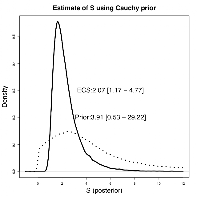
An additional factor can also be the method, in particular the choice of prior. James Annan has a recent post in which he uses a different prior to that used in some of the other analyses. It produces a 5-95% range of 1.2oC – 4.8oC, which seems mostly consistent with the IPCC range of 1.5oC – 4.5oC (which is – I think – more properly a 17-83% range). The best estimate is 2.1oC, which is maybe still a bit lower than other estimates, but still seems reasonable.
Maybe I’ll finish this post by also mentioning the recent Royal Society report which also says
value below 2oC for the lower end of the likely range of equilibrium climate sensitivity now seems less plausible.

So you do not think it’s looking like the next IPCC range is going to start at greater than 2?
I do think that the next IPCC range is probably going to start at 2oC.
What is the value of a climate model only metric, which can never be measured in the real world?
This is apparently also true for TCR as well.
Neither metric can be measured in the real world.
CO2 doubling will occur when we hit 560 ppm and we will still be fighting over what ECS and TCR ranges are.
I used to think that when we hit 560 ppm we would achieve clarity – but that assumption has been soundly rejected.
Rick,
Rather than repeating this entire discussion, I’ll just link to the other thread in which we discussed this. Starting here.
Zeke Hausfather’s post today used the Haustein et. al., 2017, simple statistical model relating forcing to observed temperatures that was the subject of a guest blog here. His main subject was the anthropogenic contribution to warming, but he also had a section on future projections:
“When provided with the radiative forcings for the RCP6.0 scenario, the simple statistical model shows warming of around 3C by 2100, nearly identical to the average warming that climate models find.”
So whether observation-based projections agree with climate model projections depends on the “observation-based” method employed.
https://www.carbonbrief.org/analysis-why-scientists-think-100-of-global-warming-is-due-to-humans
So does Gavin Schmidt.
“But the future may differ from the past, and there’s reason to think that the warming we’ve experienced so far is different from the warming to come.”
Yes, we may have a flatter slope X and the steeper slope Y later. And then an ECS and TCR for both slopes. My theory is that Y is now and X is later.
Assume Marvel’s correct. Which ECS do we use?
A ECS as low as 1.5 C is hard to imagine. We have already had a 1.2 C rise from preindustrial CO2 levels, with an additional latent temperature rise in the present TOA imbalance, around 0.9 W/m2
Olof,
Indeed. In fact, I would say that a TCR below 1.5C is now hard to imagine. Given a TCR-to-ECS ratio of about 0.6, that would also suggest an ECS of at least 2.5C.
Here’s a rather interesting discussion paper that just came online at ESD …
“Climate sensitivity estimates – sensitivity to radiative forcing time series and observational data”
https://www.earth-syst-dynam-discuss.net/esd-2017-119/
Abstract. Inferred Effective Climate Sensitivity (ECSinf) is estimated using a method combining radiative forcing (RF) time series and several series of observed ocean heat content (OHC) and near-surface temperature change in a Bayesian-framework using a simple energy balance model and a stochastic model. The model is updated compared to our previous analysis by using recent forcing estimates from IPCC, including OHC data for the deep ocean, and extending the time series to 2014. The mean value of the estimated ECSinf is 2.0 °C, with a 90 % credible interval of 1.2–3.1 °C. The mean estimate has recently been shown to be consistent with the higher values for the equilibrium climate sensitivity estimated by climate models. We show a strong sensitivity of the estimated ECSinf to the choice of a priori RF time series, excluding pre-1950 data and the treatment of OHC data. Sensitivity analysis performed by merging the upper (0–700 m) and the deep ocean OHC or using only one OHC data set (instead of four in the main analysis), both give an enhancement the mean ECSinf by about 50 % from our best estimate.
https://www.earth-syst-dynam-discuss.net/esd-2017-119/esd-2017-119.pdf“>Climate sensitivity estimates – sensitivity to radiative forcing time series and observational data
JCH,
Beat you by 32 minutes. 😉
I’ve rather suddenly developed a keen interest in ECS estimates, the pdf’s thereof, thanks mainly to JA …
Guess I missed it, but I did not see a link to the entire paper. No discussion so far.
On ECS, me too. I have carefully stayed away from it other than wondering incessantly why nobody takes the AMO out back and shoots it.
JCH,
Interesting looking paper, thanks. Amazed that they don’t seem to cite any of Nic Lewis’s work.
Everett found it.
Perhaps the authors agree there is a reason there has been such monumental skepticism and reluctant acceptance of his work at CargoCult Etc.
It just seems basic to me that if the warming hiatus that never happened was caused by a strengthening of ocean heat uptake efficiency during a period of time that coincided with Matt England’s anomalous intensified tradewinds, which both actually happened and then went away, that the observations are a bit F’d Up for primetime. So which longterm variation are they talking about? Because, as far as I can find, Matt England’s anomalous intensified tradewinds are a one-off phenomena. There is no variation to them: so far. The winds came; there was a warming hiatus in improvable datasets; the winds subsided; GMST has been shooting through the roof ever since. Anyway, I’m reading all the cloud stuff. Seems to be pointing mostly in the same direction: upward ECS.
“Interesting looking paper, thanks. Amazed that they don’t seem to cite any of Nic Lewis’s work.”
From a Google Scholar citation search of … “An objective Bayesian improved approach for applying optimal fingerprint techniques to estimate climate sensitivity”
Currently at 69 citations, including …
JA Curry, N Scafetta, C Loehle, A Parker, R McKitrick, Gervais (new one for me at least), A Ollila, M Connolly, R Connolly, RSJ Tol, J Marohasy, PJ Michaels, PC Knappenberger, WWH Soon, DR Legates, WM Briggs, Monkers, The Auditor
There are, of course, a bunch of real climate science papers, I just happened to notice a preponderance of ‘so called’ addictive authors.
Is NL a ‘so called’ gateway drug (a habit-forming author that, while not itself addictive, may lead to the use of other addictive authors)? Maybe a ‘so called’ keystone domino (but this time with real references) would be a better euphemism? 😉
See also … “Combining independent Bayesian posteriors into a confidence
distribution, with application to estimating climate sensitivity” by NL (Can’t remember if this one has already been mentioned here already).
https://www.sciencedirect.com/science/article/pii/S0378375817301702
Note to self: The JA posterior is a very close fit to a log-Pearson III distro (historically used in flood frequency analyses). My main concern is with the extremely steep (almost cliff like) front face of all these low ECS distros. Do these low ECS distros fall into a single class or parametric distro? If so, more or less, then this may negate arguments with regards to any assumed prior distro (excepting the different computed parameters thereof). I also have concerns with the observational data sets, each year adds an additional year to be considered in all these observational ECS estimates, as such, each additional year produces a different observational ECS estimate (e. g. the above mentioned discussion paper updates (their 2014 paper) through 2014, but the three highest GMST are very likely to be 2016, 2017, 2015 (in that likely order), need to lookup what will be the three highest OHC values after the 2017 data is in. Are there any papers that combine the observational data sets with the CMIP5 projections? I would think so, if so, I’d appreciate links to any papers that others here have already tripped over. TIA
EFS – the authors who have caught my eye participated in a recent meeting on clouds and sensitivity:
MD Zelinka MJ Webb P Ceppi DT McCoy DL Hartmann T Storelvmo
A 2018 abstract example:
The Climatic Impact of Thermodynamic Phase Partitioning in Mixed-Phase Clouds
Also, Andrew Dessler, SC Sherwood, and Bjorn Stevens and Mauritzen.
JCH,
An England link (or elevernteen of them) would be appreciated, say from here (Google Scholar for Matthew England) …
https://scholar.google.com/citations?hl=en&user=cND_ZAgAAAAJ&view_op=list_works&sortby=pubdate
(I’m not seeing any ECS papers by England)
Your inline text grab image is from the aforementioned discussion paper (that paper has no England references AFAICT via word search).
No, it doesn’t. That’s sort off why I want to know to what longterm variability they are referring.
This is one of their references:
Strengthening of ocean heat uptake efficiency associated with the recent climate hiatus,
This is England: the big red dive at the end of the bottom graphic:
I see these as one in the same thing; maybe that’s wrong.
JCH,
AFAIK, the discussion paper only has NH and SH OHC data, in other words not gridded, One OHC source is a reanalysis product ORAS4.
Your image is from this paper (You know this, I didn’t, so, you know, it would help if you provide a link. As a general comment/rule, I’m not sure if it is you or someone else, but whomever they are, they should not assume that others already know whatever it is that they know.) …
Click to access trade%20winds%20%26%20warming%20pause%202014.pdf
Maybe that paper is now somewhat postobsolete, given revisions to GMST before 2014 and new data since 2014 and the recent 2015-6 ENSO.
Maybe this current discussion paper is preobsolete given 2015-7 OHC and GMST time series. I’m of the opinion that there is long term variability, but that the long(er) term trends are upwards.
I did find this though …
OCEAN TEMPERATURE ANALYSIS AND HEAT CONTENT ESTIMATE FROM INSTITUTE OF ATMOSPHERIC PHYSICS
https://climatedataguide.ucar.edu/climate-data/ocean-temperature-analysis-and-heat-content-estimate-institute-atmospheric-physics
http://159.226.119.60/cheng/
http://159.226.119.60/cheng/images_files/OHC_estimate2_update2017Aug.txt
As a general concept, I like those that update their own time series (on a monthly or annual basis). But in this current discussion paper case, I’d expect a 3-year cadence: 2014, 2017 (updated through 2014), 2020 (updated through 2017), 2023 (updated through 2020), … 😦
Sorry,
Recent intensification of wind-driven circulation in the Pacific and the ongoing warming hiatus
Role of observed Pacific trade wind trends in the recent hiatus and future projections
In the data you referenced; 3rd 1/4 2017 OHC 0-700 meters; sky high. That indicates to me now ocean heat uptake may be less efficient than it was 2001 to 2014: more 0 to 700; less 700 to bottom. That could mean the IPCC SPM prediction of 2 ℃ per decade over the first two decades of the 21st century is possible, maybe even likely. It’s not that far away, through Oct; Nov and Dec will make it worse:
JCH,
RE: England’s Figure 1b. Big no-no where I come from, data ends in 2012, but the moving 20-tread trend lines continue to the very end, 2012. Therefore England must have had future data through ~2022! For a stationary system (e. g. ergodic), you have sqrt(n/(n/2))=sqrt(2) increase in uncertainty at the end of the time series (half population versus full population), for a non-stationary system (which is self evident from that figure) the uncertainty is greater than sqrt(2) at the end of that trend line (relative to a fully occupied moving average, due to additional uncertainty in the slope of the moving average)).
It also follows that, relative to the 20-year moving average, that a corresponding uncertainty can be derived from the 20-year moving average of the variance (i. e. standard deviation of the sample relative to the 20-year moving average). However that was not done or shown. There is also uncertainty in the samples themselves, so add that to the 20-year moving uncertainty.
Everett,
data ends in 2012, but the moving 20-tread trend lines continue to the very end, 2012.
The x-axis year is actually the end of the trend period, I guess for easy visual comparison with the graph above it and the anomaly data on the same figure, so the last datapoints relate to 1993-2012 trends. The ERA data begins in 1979.
paulski0,
OK, I see. A 20-year trend isn’t a 20-year moving average. D’oh! I guess it also helps to properly read the caption. My bad. Thanks.
On another, oh look, a squirrel gambit, it appears that the ECMWF is now at ORAS5 …
Click to access Zuo_RMetSDASIG_Mar2017.pdf
Magdalena A Balmaseda
https://scholar.google.com/citations?hl=en&user=Buz0VmAAAAAJ&view_op=list_works&sortby=pubdate
Everett/others –In case you missed it, SoD has a post about two of the recent papers on clouds.
Figure from Ceppi:
JCH,
Did you mean the 2017-12-24 SOD post?
Your link is to the previous SOD post but your figure above is from the current SOD post.
Clouds and Water Vapor – Part Eleven – Ceppi et al & Zelinka et al
Yes, Part Eleven. On the prior thread I started posting links to recent papers by the authors, plus Dessler, mentioned above, and pretty soon Professor Dessler showed up. Then it degraded into the usual nonsense, but SoD must have found it interesting. My sense is these guys are about to narrow the sensitivity range, maybe both ends.
The influence of internal variability on Earth’s energy balance framework and implications for
2 estimating climate sensitivity Dessler; Mauritsen; Stevens
It’s a discussion paper.
Pingback: Confounding ECS estimates | …and Then There's Physics